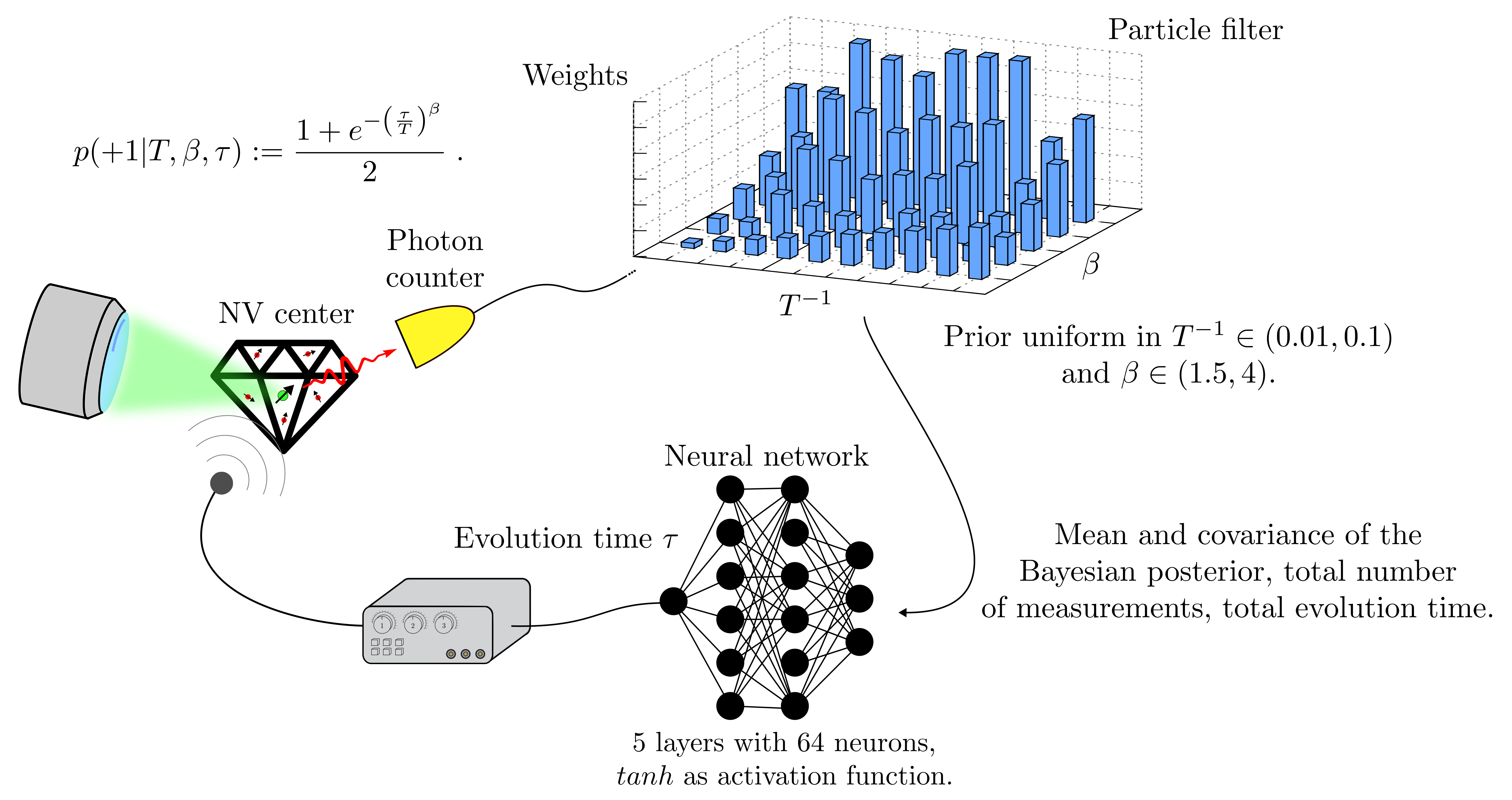
Examples
NV center - DC Magnetometry
- class Magnetometry(particle_filter: ParticleFilter, phys_model: NVCenter, control_strategy: Callable, simpars: SimulationParameters, cov_weight_matrix=None, eta_flag: bool = False, extraction_flag: bool = False, cov_flag: bool = False)
Bases:
StatelessMetrologySimulates the estimation of a magnetic field with a mean square error loss. This class is suitable for a neural network agent, for a static strategy, and for other simple controls known in the literature, like the
 strategy
and the particle guess heuristic (PGH).
It works both for static and for oscillating
magnetic fields.
strategy
and the particle guess heuristic (PGH).
It works both for static and for oscillating
magnetic fields.Constructor of the
Magnetometryclass.Parameters
- particle_filter:
ParticleFilter Particle filter responsible for the update of the Bayesian posterior on the parameters and on the state of the probe. It contains the methods for applying the Bayes rule and computing Bayesian estimators from the posterior.
- phys_model:
NVCenter Abstract description of the parameters encoding and of the measurement on the NV center.
- control_strategy: Callable
Callable object (normally a function or a lambda function) that computes the values of the controls for the next measurement from the Tensor input_strategy. This class expects a callable with the following header
controls =
control_strategy(input_strategy)
It is typically a wrapper for the neural network or a vector of static controls.
- simpars:
SimulationParameters Contains the flags and parameters that regulate the stopping condition of the measurement loop and modify the loss function used in the training.
- cov_weight_matrix: List, optional
Weight matrix that determines the relative contribution to the total error of the parameters in phys_model.params. It is list of float representing a positive semidefinite matrix. If this parameter is not passed then the default weight matrix is the identity, i.e.
 .
.- eta_flag: bool = False
This flag controls the addition of a normalization factor to the MSE loss.
If eta_flag is True, the MSE loss is divided by the normalization factor
(56)

where
 are the bounds
of the i-th parameter in phys_model.params
and
are the bounds
of the i-th parameter in phys_model.params
and  are the diagonal entries of
cov_weight_matrix.
are the diagonal entries of
cov_weight_matrix.  is the total
elapsed evolution time, which can be different
for each estimation in the batch.
is the total
elapsed evolution time, which can be different
for each estimation in the batch.Achtung! This flag should be used only if the resource is the total estimation time.
- extraction_flag: bool = False
If extraction_flag=True a couple of particles are sampled from the posterior and added to the input_strategy Tensor. This is useful to simulate the PGH control for the evolution time, according to which the k-th control should be
(57)

with
 ,
where
,
where  and
and  are
respectively the first and the second particle
extracted from the ensemble and
are
respectively the first and the second particle
extracted from the ensemble and  is the cartesian norm.
- cov_flag: bool = False
If cov_flag=True a flattened version of the covariance matrix of the particle filter ensemble is added to the input_strategy Tensor. This is useful to simulate the
control strategy and its variant that accounts
for a finite
transversal relaxation time. They prescribe
respectively for the k-th control(58)
![\tau_k = \frac{1}{\left[ \text{tr}
(\Sigma) \right]^{\frac{1}{2}} } \; ,](_images/math/33b57154d4dbfb3e8335d633a060ec0d48a73dc7.svg)
and
(59)
![\tau_k = \frac{1}{\left[ \text{tr}
(\Sigma) \right]^{\frac{1}{2}} +
\widehat{T_2^{-1}}} \; ,](_images/math/21eb09b7a501b0c32c5f1a8beb903e794b525e4d.svg)
being
 the covariance matrix
of the posterior computed with the
the covariance matrix
of the posterior computed with the
compute_covariance()method.
- generate_input(weights: Tensor, particles: Tensor, meas_step: Tensor, used_resources: Tensor, rangen: Generator)
Generates the input_strategy Tensor of the
generate_input()method. The returned Tensor is influenced by the parameters extract_flag and cov_flag of the constructor.
- loss_function(weights: Tensor, particles: Tensor, true_values: Tensor, used_resources: Tensor, meas_step: Tensor)
Mean square error on the parameters, as computed in
loss_function(). The behavior of this method is influence by the flag eta_flag passed to the constructor of the class.
- particle_filter:
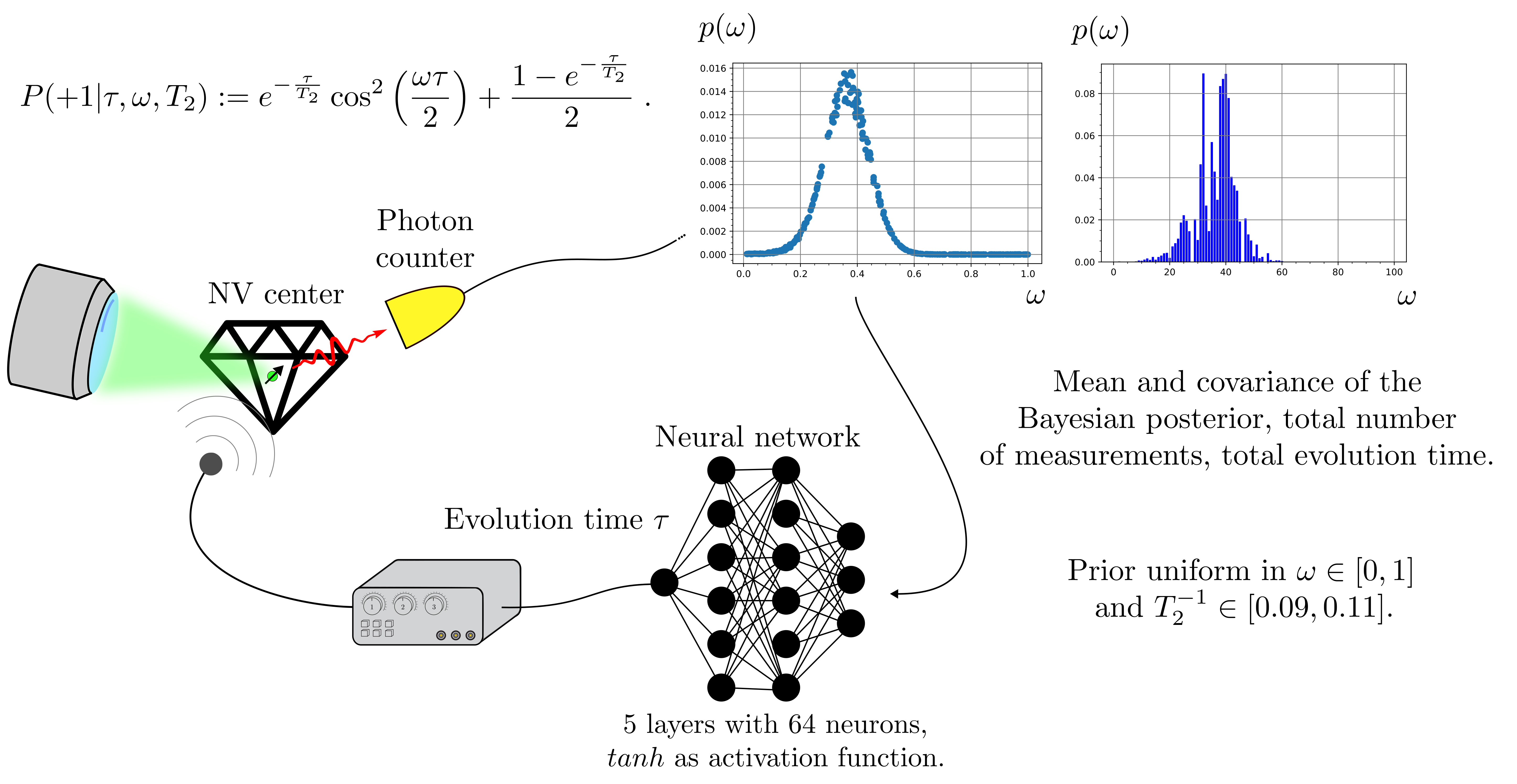
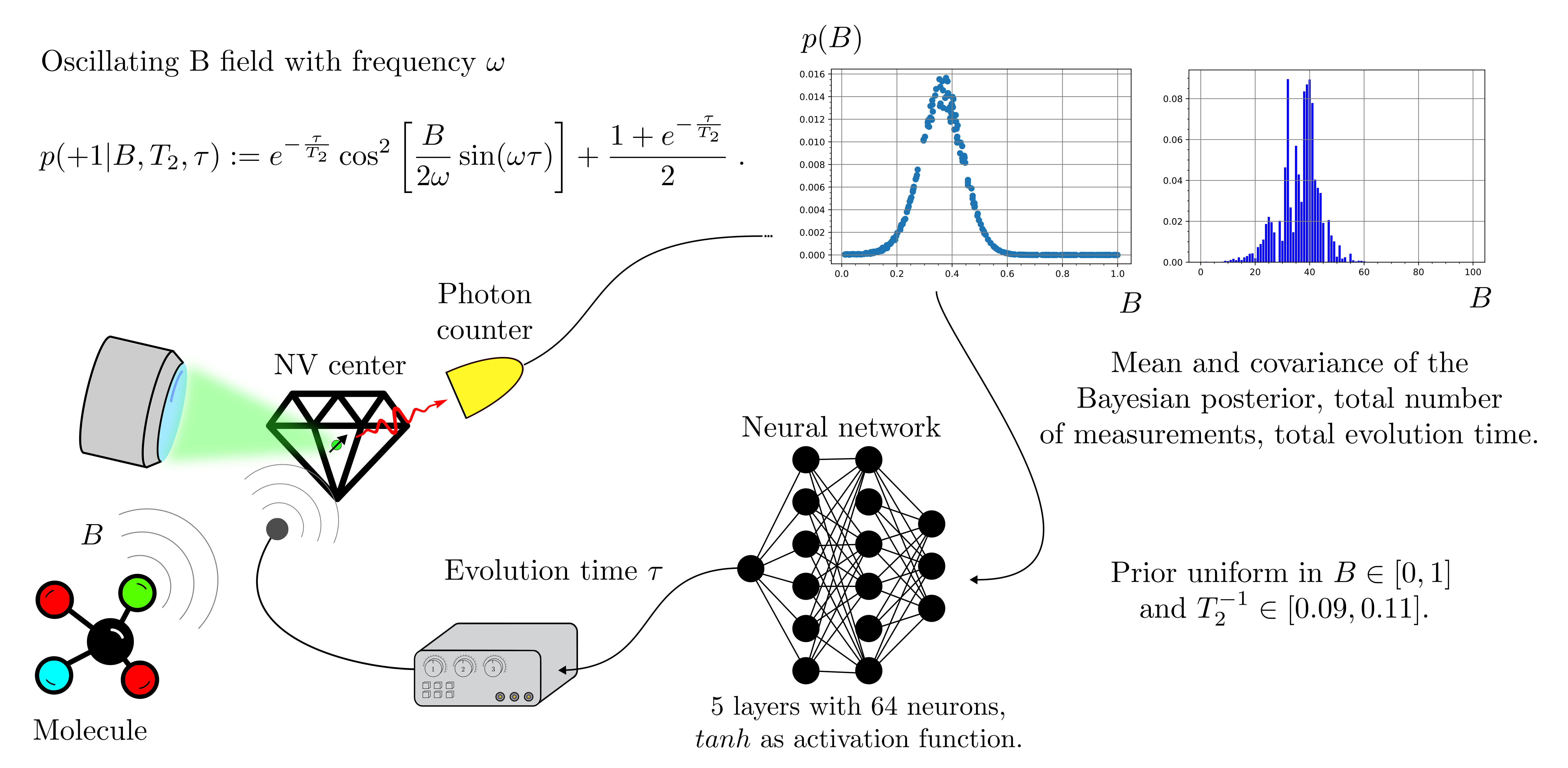
- class NVCenter(batchsize: int, params: List[Parameter], prec: Literal['float64', 'float32'] = 'float64', res: Literal['meas', 'time'] = 'meas', control_phase: bool = False)
Bases:
StatelessPhysicalModelModel for the negatively charged NV center in diamond used for various quantum metrological task. A single measurement on the NV center consists in multiple Ramsey sequencies of the same controllable duration applied to the NV center, followed by photon counting of the photoluminescent photon and a majority voting to decide the binary outcome. The NV center is reinitialized after each photon counting. During the free evolution in the Ramsey sequence the NV center precesses freely in the external magnetic field, thereby encoding its value in its state. The two possible controls we have on the system are the duration of the free evolution
 and the phase
 applied before
the photon counting.
The resource of the estimation task
can be either the total number of measurements or
the total evolution time.
applied before
the photon counting.
The resource of the estimation task
can be either the total number of measurements or
the total evolution time.Achtung! The
model()method must still be implemented in this class. It should describe the probability of getting in the measurement after the majority voting
from the collected photons.
in the measurement after the majority voting
from the collected photons.Constructor of the
NVCenterclass.Parameters
- batchsize: int
Batchsize of the simulation, i.e. number of estimations executed simultaneously.
- params: List[
Parameter] List of unknown parameters to estimate in the NV center experiment, with their respective bounds.
- prec{“float64”, “float32”}
Precision of the floating point operations in the simulation.
- res: {“meas”, “time”}
Resource type for the present metrological task, can be either the total evolution time, i.e. time, or the total number of measurements on the NV center, i.e. meas.
- control_phase: bool = False
If this flag is True, beside the free evolution time, also the phase applied before the photon counting is controlled by the agent.
- count_resources(resources: Tensor, outcomes: Tensor, controls: Tensor, true_values: Tensor, meas_step: Tensor)
The resources can be either the total number of measurements, or the total evolution time, according to the attribute res of the
NVCenterclass.
- perform_measurement(controls: Tensor, parameters: Tensor, meas_step: Tensor, rangen: Generator) Tuple[Tensor, Tensor]
Measurement on the NV center.
The NV center is measured after having evolved freely in the magnetic field for a time specified by the parameter control. The possible outcomess are
and  ,
selected stochastically according to the probabilities
,
selected stochastically according to the probabilities
 , where is the
evolution time (the control) and
, where is the
evolution time (the control) and  the parameters to estimate. This method
returns the observed outcomes
and their log-likelihood.
the parameters to estimate. This method
returns the observed outcomes
and their log-likelihood.Achtung! The
model()method must return the probability
- class NVCenterDCMagnetometry(batchsize: int, params: List[Parameter], prec: Literal['float64', 'float32'] = 'float64', res: Literal['meas', 'time'] = 'meas', invT2: Optional[float] = None)
Bases:
NVCenterModel describing the estimation of a static magnetic field with an NV center used as magnetometer. The spin-spin relaxation time
 can
be either known, or be a parameter to
estimate. The estimation will be
formulated in terms of the precession
frequency
can
be either known, or be a parameter to
estimate. The estimation will be
formulated in terms of the precession
frequency  of the NV center, which
is proportional to the magnetic
field
of the NV center, which
is proportional to the magnetic
field  .
.This physical model and the application of Reinforcement Learning to the estimation of a static magnetic fields have been also studied in the seminal work of Fiderer, Schuff and Braun 1.
Constructor of the
NVCenterDCMagnetometryclass.Parameters
- batchsize: int
Batchsize of the simulation, i.e. number of estimations executed simultaneously.
- params: List[
Parameter] List of unknown parameters to estimate in the NV center experiment, with their respective bounds.
- prec{“float64”, “float32”}
Precision of the floating point operations in the simulation.
- res: {“meas”, “time”}
Resource type for the present metrological task, can be either the total evolution time, i.e. time, or the total number of measurements on the NV center, i.e. meas.
- invT2: float, optional
If this parameter is specified only the precession frequency
is considered as an unknown
parameter, while the inverse of the
transverse relaxation time is fixed
to the value invT2. In this case the list params
must contain a single parameter, i.e. omega.
If no invT2 is specified,
it is assumed that it is an unknown parameter that
will be estimated along the frequency in the Bayesian
procedure. In this case params must contain two
objects, the second of them should be the inverse of the
transversal relaxation time.
- model(outcomes: Tensor, controls: Tensor, parameters: Tensor, meas_step: Tensor, num_systems: int = 1) Tensor
Model for the outcome of a measurement on a NV center subject to free precession in a static magnetic field. The probability of getting the outcome
is(60)

The evolution time
is controlled
by the trainable agent, and
is the unknown precession frequency, which is
proportional to the magnetic field.
The parameter  may or may not be an unknown in the estimation,
according to the value of the attribute invT2
of the
may or may not be an unknown in the estimation,
according to the value of the attribute invT2
of the NVCenterDCMagnetometryclass.
- main()
Runs the same simulations done by Fiderer, Schuff and Braun 1.
The performances of the optimized neural network and static strategies are reported in the following plot, together with other strategies commonly used in the literature. The resources can be the number of measurements or the total evolution time.
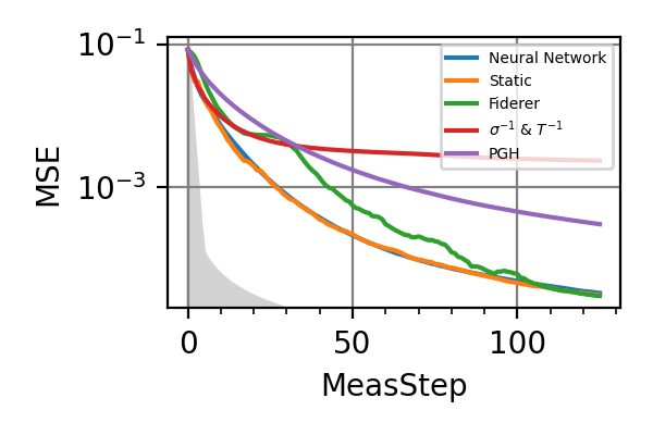
Fig. 1 invT2=0.01, Meas=128
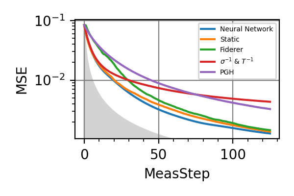
Fig. 2 invT2=0.1, Meas=128
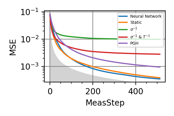
Fig. 3 invT2 in (0.09, 0.11), Meas=512
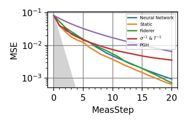
Fig. 4 invT2=0, Meas=24
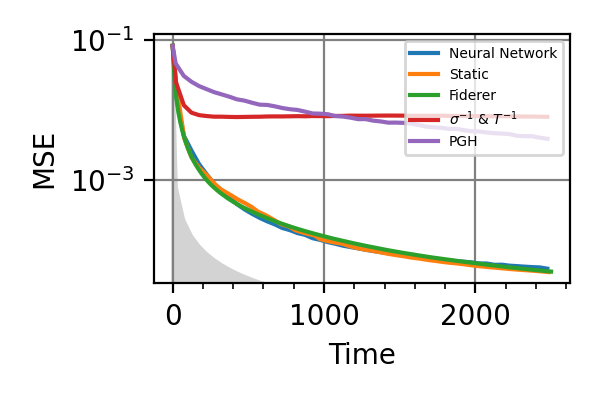
Fig. 5 invT2=0.01, Time=2560
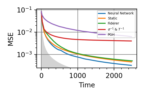
Fig. 6 invT2=0.1, Time=2560
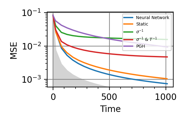
Fig. 7 invT2 in (0.09, 0.11), Time=1024
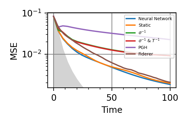
Fig. 8 invT2=0, Time=128
For the plot referring to the estimation of omega only the green line is the best performance found in the literature so far, obtained in 1 with model-free RL. In the plot corresponding to the simultaneous estimation of both the frequency and the decoherence time we din’t compare our results with 1 and the green line in simply the
.The shaded grey areas in the above plot indicate the Bayesian Cramér-Rao bound, which is the the ultimate precision bound computed from the Fisher information.
From the above plots we can conclude that the adaptive strategy offers no advantage with respect to the optimal static strategy for those experiments limited in the number of measurements and for all those with a sufficiently high coherence time. For
 we
see some small advantage of the adaptive
strategy in the time limited experiments.
This observation is in accordance with
the analysis based only on the Fisher information.
For
we
see some small advantage of the adaptive
strategy in the time limited experiments.
This observation is in accordance with
the analysis based only on the Fisher information.
For  the Fisher information
of a single measurement is
the Fisher information
of a single measurement is  and is
independent on . For
and is
independent on . For  the Fisher information manifests a dependence
on , which could indicate
the possibility of an adaptive strategy
being useful, which is confirmed in
these simulations.
the Fisher information manifests a dependence
on , which could indicate
the possibility of an adaptive strategy
being useful, which is confirmed in
these simulations.Notes
The results of the simulations with invT2 in (0.09, 0.11) are very similar to that with invT2=0.1 because of the relatively narrow prior on invT2.
For an NV center used as a magnetometer the actual decoherence model is given by
 instead of

Achtung! The performances of the time limited estimations with the
and the PGH strategies are not in accordance
with the results of
Fiderer, Schuff and Braun 1. Also the simulations
with invT2 in (0.09, 0.11) do not agree with the results
reported in this paper.Normally in the applications the meaningful resource is the total time required for the estimation. This doesn’t coincide however with the total evolution time that we considered, because the initialization of the NV center, the read-out the and the data processing all take time. This overhead time is proportional to the number of measurements, so that in a real experiment we expect the actual resource to be a combination of the evolution time and the number of measurements.
In a future work the role of the higher moments of the posterior distribution in the determination of the controls should be explored. In particular it should be understood if with
(61)

more advantage from the adaptivity could be extracted.
In room-temperature magnetometry it is impossible to do single-shot readout of the NV center state (SSR). We should train the control strategy to work with non-SSR, as done by Zohar et al 2
All the trainings of this module have been done on a GPU NVIDIA Tesla V100-SXM2-32GB, each requiring
 hours.
- 2
I Zohar et al, Quantum Sci. Technol. 8 035017 (2023).
- parse_args()
Arguments
- scratch_dir: str
Directory in which the intermediate models should be saved alongside the loss history.
- trained_models_dir: str = “./nv_center_dc/trained_models”
Directory in which the finalized trained model should be saved.
- data_dir: str = “./nv_center_dc/data”
Directory containing the csv files produced by the
performance_evaluation()and thestore_input_control()functions.- prec: str = “float32”
Floating point precision of the whole simulation.
- n: int = 64
Number of neurons per layer in the neural network.
- num_particles: int = 480
Number of particles in the ensemble representing the posterior.
- iterations: int = 32768
Number of training steps.
- scatter_points: int = 32
Number of points in the Resources/Precision csv produced by
performance_evaluation().
- static_field_estimation(args, batchsize: int, max_res: float, learning_rate: float = 0.01, gradient_accumulation: int = 1, cumulative_loss: bool = False, log_loss: bool = False, res: Literal['meas', 'time'] = 'meas', invT2: Optional[float] = None, invT2_bound: Optional[Tuple] = None, cov_weight_matrix: Optional[List] = None, omega_bounds: Tuple[float, float] = (0.0, 1.0))
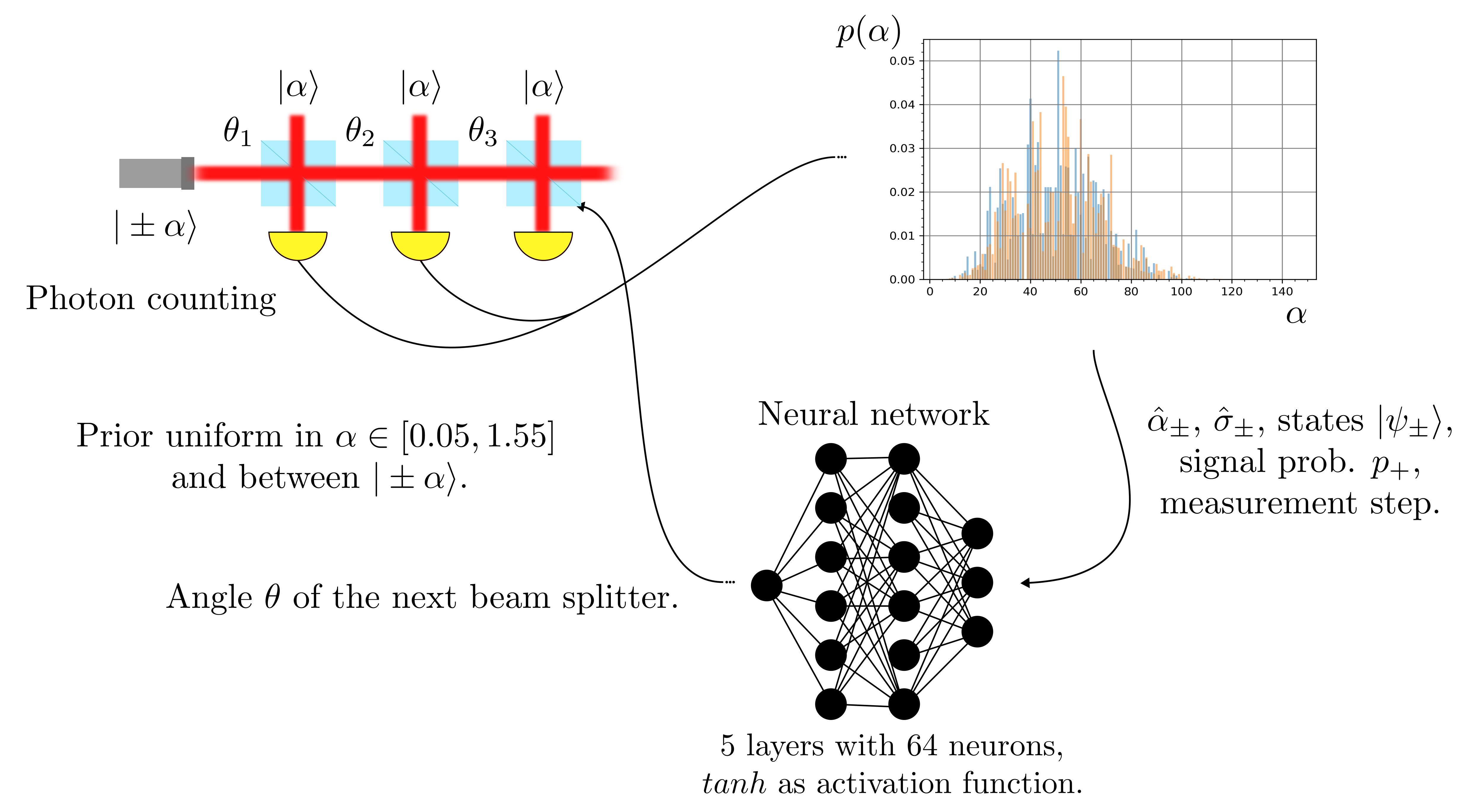
Simulates the Bayesian estimation of a static magnetic field with an NV center, for a neural network controlling the evolution time, a static strategy, two variations of the
strategy, and the
particle guess heuristic (PGH).The measurement loop is showed in the following picture.
Parameters
- args:
Arguments passed to the Python script.
- batchsize: int
Batchsize of the simulation, i.e. number of estimations executed simultaneously.
- max_res: float
Maximum amount of resources allowed to be consumed in the estimation.
- learning_rate: float = 1e-2
Initial learning rate for the neural network. The initial learning rate of the static strategy is fixed to 1e-1. They both decay with
InverseSqrtDecay.- gradient_accumulation: int = 1
Flag of the
train()function.- cumulative_loss: bool = False
Flag
cumulative_loss.- log_loss: bool = False
Flag
log_loss.- res: {“meas”, “time”}
Type of resource for the simulation. It can be either the number of measurements or the total evolution time.
- invT2: float, optional
Inverse of the transversal relaxation time. If
 or it is unknown and must
be estimated, this parameter should not
be passed.
or it is unknown and must
be estimated, this parameter should not
be passed.- invT2_bound: Tuple[float, float], optional
Extrema of the uniform prior for the Bayesian estimation of the inverse of the transversal relaxation time.
- cov_weight_matrix: List, optional
Weight matrix for the mean square error on the frequency and on the inverse of the coherence time
.- omega_bounds: Tuple[float, float] = (0.0, 1.0)
Extrema of admissible values for the precession frequency.
NV center - Phase control
- class NVCenterDCMagnPhase(batchsize: int, params: List[Parameter], prec: Literal['float64', 'float32'] = 'float64', res: Literal['meas', 'time'] = 'meas', invT2: Optional[float] = None)
Bases:
NVCenterModel describing the estimation of a static magnetic field with an NV center used as magnetometer. The transversal relaxation time
can
be either known, or be a parameter to
estimate. The estimation will be
formulated in terms of the precession
frequency of the NV center, which
is proportional to the magnetic
field .
With respect to the nv_center_dcmodule we add here the possibility of imprinting an arbitrary phase on the NV-center state before the photon counting measurement.Constructor of the
NVCenterDCMagnPhaseclass.Parameters
- batchsize: int
Batchsize of the simulation, i.e. number of estimations executed simultaneously.
- params: List[
Parameter] List of unknown parameters to estimate in the NV center experiment, with their respective bounds. This contains either the precession frequency only or the frequency and the inverse coherence time.
- prec{“float64”, “float32”}
Precision of the floating point operations in the simulation.
- res: {“meas”, “time”}
Resource type for the present metrological task, can be either the total evolution time, i.e. time, or the total number of measurements on the NV center, i.e. meas.
- invT2: float, optional
If this parameter is specified only the precession frequency
is considered as an unknown
parameter, while the inverse of the
transverse relaxation time is fixed
to the value invT2. In this case the list params
must contain a single parameter, i.e. omega.
If no invT2 is specified,
it is assumed that it is an unknown parameter that
will be estimated along the frequency in the Bayesian
procedure. In this case params must contain two
objects, the second of them should be the inverse of the
transversal relaxation time.
- model(outcomes: Tensor, controls: Tensor, parameters: Tensor, meas_step: Tensor, num_systems: int = 1) Tensor
Model for the outcome of a measurement on a NV center that has been precessing in a static magnetic field. The probability of getting the outcome
is(62)

The evolution time
and
the phase are controlled
by the trainable agent, and
is the unknown precession frequency, which is
proportional to the magnetic field.
The parameter
may or may not be an unknown in the estimation,
according to the value of the attribute invT2
of the NVCenterDCMagnPhaseclass.
- main()
Runs the same simulations done by Fiderer, Schuff and Braun 1 but with the possibility of controlling the phase of the NV center before the Ramsey measurement.
The performances of the optimized neural network and the static strategy are reported in the following plots, together with other strategies commonly used in the literature. The resource can be either the total number of measurements or the total evolution time. Beside the NN optimized to control
and
, the
performances of the NN trained to control
only the evolution time are reported in
brown.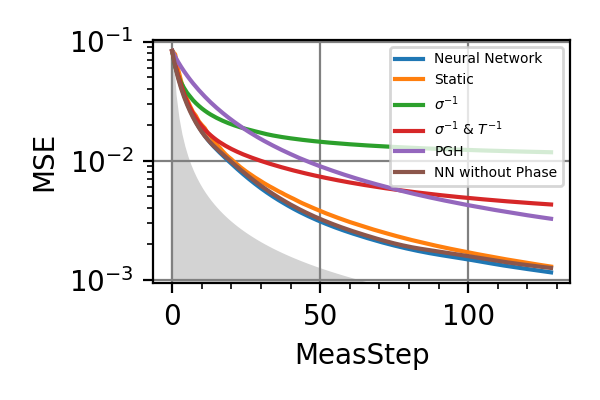
Fig. 9 invT2=0.1, Meas=128
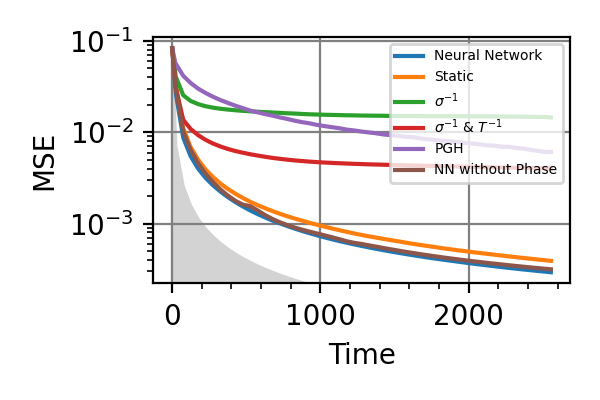
Fig. 10 invT2=0.1, Time=2560
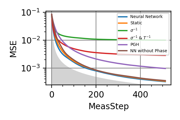
Fig. 11 invT2 in (0.09, 0.11), Meas=512
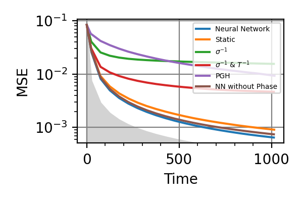
Fig. 12 invT2 in (0.09, 0.11), Time=1024
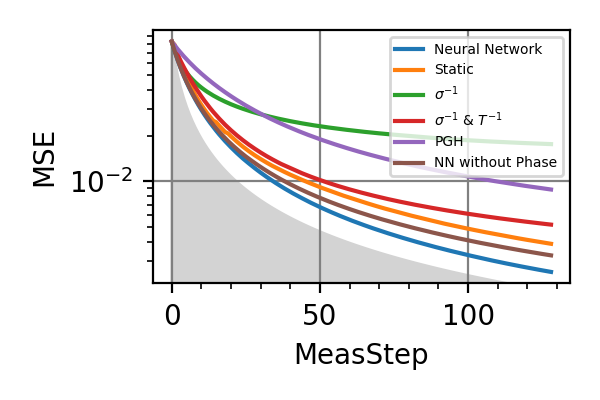
Fig. 13 invT2=0.2, Meas=128
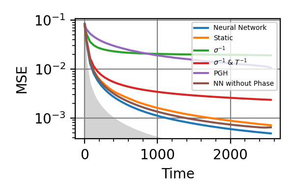
Fig. 14 invT2=0.2, Time=2560
The shaded grey areas in the above plot indicate the Bayesian Cramér-Rao bound, which is the the ultimate precision bound computed from the Fisher information.
There is only a very small advantage in controlling the phase for
 , if there is any at all.
Similarly, with
, if there is any at all.
Similarly, with  no advantage has
been found. For and Time=2560 the
phase control had converged to
no advantage has
been found. For and Time=2560 the
phase control had converged to  , and
more training could not take it out of this minimum.
For
, and
more training could not take it out of this minimum.
For  the advantage in introducing
also the phase control becomes more consistent.
the advantage in introducing
also the phase control becomes more consistent.Notes
For the phase control be advantageous, the phase
 must be known to some extent.
While the error on goes down, the
evolution time increases, so that the error on
doesn’t go to zero. This limits
the utility of controlling the phase in
DC magnetometry.
must be known to some extent.
While the error on goes down, the
evolution time increases, so that the error on
doesn’t go to zero. This limits
the utility of controlling the phase in
DC magnetometry.All the training of this module have been done on a GPU NVIDIA Tesla V100-SXM2-32GB, each requiring
hours.
- parse_args()
Arguments
- scratch_dir: str
Directory in which the intermediate models should be saved alongside the loss history.
- trained_models_dir: str = “./nv_center_dc_phase/trained_models”
Directory in which the finalized trained model should be saved.
- data_dir: str = “./nv_center_dc_phase/data”
Directory containing the csv files produced by the
performance_evaluation()and thestore_input_control()functions.- prec: str = “float32”
Floating point precision of the whole simulation.
- n: int = 64
Number of neurons per layer in the neural network.
- num_particles: int = 480
Number of particles in the ensemble representing the posterior.
- iterations: int = 32768
Number of training steps.
- scatter_points: int = 32
Number of points in the Resources/Precision csv produced by
performance_evaluation().
- static_field_estimation(args, batchsize: int, max_res: float, learning_rate: float = 0.01, gradient_accumulation: int = 1, cumulative_loss: bool = False, log_loss: bool = False, res: Literal['meas', 'time'] = 'meas', invT2: Optional[float] = None, invT2_bound: Optional[Tuple] = None, cov_weight_matrix: Optional[List] = None, omega_bounds: Tuple[float, float] = (0.0, 1.0))
Simulates the Bayesian estimation of a static magnetic field with an NV center, for a neural network controlling the sensor, a static strategy, two variations of the
strategy, and the
particle guess heuristic (PGH). Beside
the evolution time also the phase
is be controlled by the agent.Parameters
- args:
Arguments passed to the Python script.
- batchsize: int
Batchsize of the simulation, i.e. number of estimations executed simultaneously.
- max_res: float
Maximum amount of resources allowed to be consumed in the estimation.
- learning_rate: float = 1e-2
Initial learning rate for the neural network. The initial learning rate of the static strategy is fixed to 1e-1. They both decay with
InverseSqrtDecay.- gradient_accumulation: int = 1
Flag of the
train()function.- cumulative_loss: bool = False
Flag
cumulative_loss.- log_loss: bool = False
Flag
log_loss.- res: {“meas”, “time”}
Type of resource for the simulation. It can be either the number of Ramsey measurements or the total evolution time.
- invT2: float, optional
Inverse of the transversal relaxation time. If
or it is unknown and must
be estimated, this parameter should not
be passed.- invT2_bound: Tuple[float, float], optional
Extrema of the uniform prior for the Bayesian estimation of the inverse of the transversal relaxation time.
- cov_weight_matrix: List, optional
Weight matrix for the mean square error on the frequency and on the inverse of the coherence time
.- omega_bounds: Tuple[float, float] = (0.0, 1.0)
Extrema of admissible values for the precession frequency.
NV center - AC Magnetometry
- class NVCenterACMagnetometry(batchsize: int, params: List[Parameter], omega: float = 0.2, prec: Literal['float64', 'float32'] = 'float64', res: Literal['meas', 'time'] = 'meas', invT2: Optional[float] = None)
Bases:
NVCenterThis model describes the estimation of the intensity of oscillating magnetic field of known frequency with an NV center used as magnetometer. The transversal relaxation time
can
be either known, or be a parameter to
estimate.Constructor of the
NVCenterACMagnetometryclass.Parameters
- batchsize: int
Batchsize of the simulation, i.e. number of estimations executed simultaneously.
- params: List[
Parameter] List of unknown parameters to estimate in the NV center experiment, with their respective bounds. This contains either the field intensity
only or
and the inverse coherence time .- omega: float = 0.2
Frequency of the oscillating magnetic field to be estimated.
- prec{“float64”, “float32”}
Precision of the floating point operations in the simulation.
- res: {“meas”, “time”}
Resource type for the present metrological task, can be either the total evolution time, i.e. time, or the total number of measurements on the spin, i.e. meas.
- invT2: float, optional
If this parameter is specified the estimation is performed only for the field intensity
while the inverse of the
transverse relaxation time is fixed
to the value invT2. In this case the list params
must contain a single parameter.
If no invT2 is specified,
it is assumed that it is an unknown parameter that
will be estimated along by the Bayesian
procedure. In this case params must contain two
objects, the second of them should be the inverse of the
transversal relaxation time.
- model(outcomes: Tensor, controls: Tensor, parameters: Tensor, meas_step: Tensor, num_systems: int = 1)
Model for the outcome of a measurement on a spin that has been precessing in an oscillating magnetic field of intensity
and known frequency
omega. The probability of getting the
outcome is(63)
![p(+1|B, T_2, \tau) := e^{-\frac{\tau}{T_2}}
\cos^2 \left[ \frac{B}{2 \omega} \sin( \omega \tau)
\right] + \frac{1-e^{-\frac{\tau}{T_2}}}{2} \; .](_images/math/3b4a82a64f68d27714aff93e09fa1440727f0f84.svg)
The evolution time
is controlled
by the trainable agent, and
is the unknown magnetic field.
The parameter
may or may not be an unknown in the estimation,
according to the value of the attribute invT2
of the NVCenterACMagnetometryclass.
- alternate_field_estimation(args, batchsize: int, max_res: float, learning_rate: float = 0.01, gradient_accumulation: int = 1, cumulative_loss: bool = False, log_loss: bool = False, res: Literal['meas', 'time'] = 'meas', omega: float = 0.2, invT2: Optional[float] = None, invT2_bound: Optional[Tuple] = None, cov_weight_matrix: Optional[List] = None, B_bounds: Tuple[float, float] = (0.0, 1.0))
Simulates the Bayesian estimation of the intensity of an oscillating magnetic field of known frequency with an NV center sensor, for a neural network controlling the evolution time, a static strategy, two variations of the
strategy, and the
particle guess heuristic (PGH).The measurement loop is showed in the following picture.
Parameters
- args:
Arguments passed to the Python script.
- batchsize: int
Batchsize of the simulation, i.e. number of estimations executed simultaneously.
- max_res: float
Maximum amount of resources allowed to be consumed in the estimation.
- learning_rate: float = 1e-2
Initial learning rate for the neural network. The initial learning rate of the static strategy is fixed to 1e-1. They both decay with
InverseSqrtDecay.- gradient_accumulation: int = 1
Flag of the
train()function.- cumulative_loss: bool = False
Flag
cumulative_loss.- log_loss: bool = False
Flag
log_loss.- res: {“meas”, “time”}
Type of resource for the simulation. It can be either the number of measurements or the total evolution time.
- omega: float = 0.2
Known frequency of the oscillating magnetic field.
- invT2: float, optional
Inverse of the transversal relaxation time. If it is infinity or it is unknown and must be estimated, this parameter should not be passed.
- invT2_bound: Tuple[float, float], optional
Extrema of admissible values of the inverse of the transversal relaxation time, whose precise value is not known before the estimation.
- cov_weight_matrix: List, optional
Weight matrix for the mean square error on the field intensity and on the decoherence parameter.
- B_bounds: Tuple[float, float] = (0.0, 1.0)
Extrema of admissible values for the intensity of the magnetic field.
- main()
Runs the simulations for the estimation of the intensity of an oscillating magnetic field of known frequency, for the same parameters of the simulations done by Fiderer, Schuff and Braun 1,
The performances of the optimized neural network and static strategies are reported in the following plots, together with the simulated
and PGH strategies, for a range of resources
and coherence times. The resource can be either
the total evolution time or the total
number of measurements.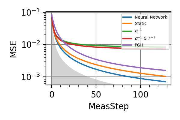
Fig. 15 invT2=0.01, Meas=128
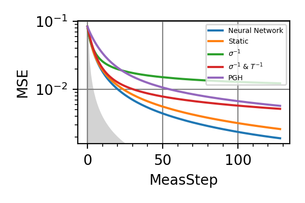
Fig. 16 invT2=0.1, Meas=128
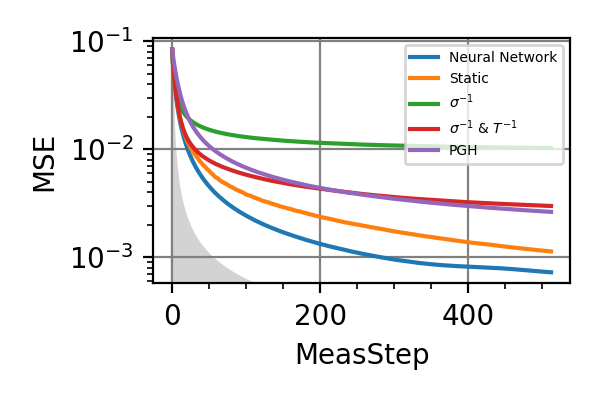
Fig. 17 invT2 in (0.09, 0.11), Meas=512
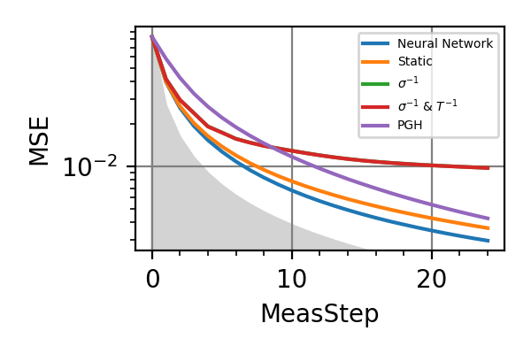
Fig. 18 invT2=0, Meas=24
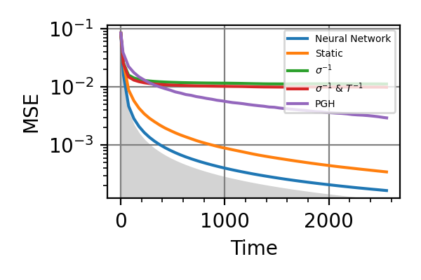
Fig. 19 invT2=0.01, Time=2560
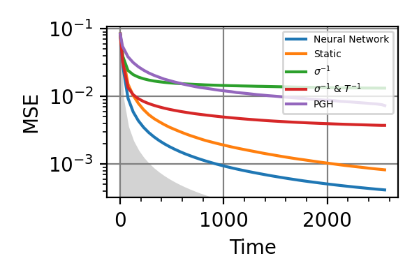
Fig. 20 invT2=0.1, Time=2560
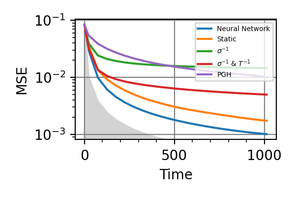
Fig. 21 invT2 in (0.09, 0.11), Time=1024
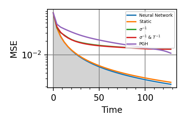
Fig. 22 invT2=0, Time=128
The shaded grey areas in the above plot indicate the Bayesian Cramér-Rao bound, which is the the ultimate precision bound computed from the Fisher information.
In all simulations we see that an “adaptivity-gap” opens between the precision of the static and the NN strategies as the resources grow.
Notes
The model used in this example is formally equivalent to that of the
nv_center_dcmodule, where the adaptive strategy gives only small advantages, at difference with the results obtained hare for AC-magnetometry. This is because the AC model maps to the DC one in a very different region of parameters with respect to the region we have explored innv_center_dc.In AC magnetometry the technique of dynamical decoupling (DD) is often used to improve the sensitivity with respect to
and to increase the coherence
time . This consists in series
of  -pulses that reverse the
sign of the accumulated phase.
Given
-pulses that reverse the
sign of the accumulated phase.
Given  the times
at which the instantaneous -pulse
are applied, the outcome probability for
a noiseless estimation is given by
the times
at which the instantaneous -pulse
are applied, the outcome probability for
a noiseless estimation is given by(64)
![p(0|B, T_2, \lbrace t_i \rbrace) = \cos^2 \left[ \frac{B}{2 \omega}
\sum_{i=1}^{N+1} (-1)^i \left[ \sin(\omega t_{i})-
\sin(\omega t_{i-1}) \right] \right] \; ,](_images/math/b4d4c2127b454b28a1f0163e4fd53809a1c2507d.svg)
with
 being the number of pulses,
and
being the number of pulses,
and  and
and  being respectively
the initialization and the measurement times.
being respectively
the initialization and the measurement times.In the simulations done we have used no
-pulse,
but optimizing their application is the natural
extension of this example, left
for future works. For controlling the pulses
there are possibilities:the interval between the pulses is fixed to
 , which is
produced by a NN together with the
number of pulses N,
, which is
produced by a NN together with the
number of pulses N,the controls are the
time
intervals  .
The number of pulses is fixed but they
can be made ineffective with
.
The number of pulses is fixed but they
can be made ineffective with  ,
,the control is the free evolution time
together with a boolean variable, that tells
whether a pulse or a measurement has to be applied after
the free evolution. This would require a stateful model
for the NV center, where the current phase is
the state.
The problem of estimating
knowing
the frequency is complementary to the
protocol for the optimal discrimination of
frequencies presented in 3, which is used
to distinguish chemical species in a sample.
In this work
the authors put forward an optimal strategy
for the discrimination of two frequencies
and  ,
knowing the intensity .
If
,
knowing the intensity .
If  and
the field intensity is unknown a two stage approach
to the problem is possible.
We can estimate as done in this example,
i.e. by considering the frequency fixed to
, and then proceed with the optimal
frequency discrimination based on the intensity
just estimated. The error probability of the second
stage depends on the precision
of the first. Given a fixed total time for the discrimination,
the time assigned to the first and the
second stage can be optimized to minimize the
final error. For close frequencies we
expect this two stage protocol to be
close to optimality. A small improvement would
be to simulate the estimation of
with the frequency as a nuisance parameters.
It is important for the first stage, the estimation
of the field intensity, to have low sensitivity
to variations in the frequency.
For optimizing frequency discrimination
with as a nuisance parameter
in a fully integrated protocol the introduction
of -pulses is necessary, just like
for dynamical decoupling.
The natural extension of hypothesis testing
on the frequency is the
estimation of both the intensity and the frequency
of the magnetic field optimally, both starting from
a broad prior. All these improvements are left
for future work.
and
the field intensity is unknown a two stage approach
to the problem is possible.
We can estimate as done in this example,
i.e. by considering the frequency fixed to
, and then proceed with the optimal
frequency discrimination based on the intensity
just estimated. The error probability of the second
stage depends on the precision
of the first. Given a fixed total time for the discrimination,
the time assigned to the first and the
second stage can be optimized to minimize the
final error. For close frequencies we
expect this two stage protocol to be
close to optimality. A small improvement would
be to simulate the estimation of
with the frequency as a nuisance parameters.
It is important for the first stage, the estimation
of the field intensity, to have low sensitivity
to variations in the frequency.
For optimizing frequency discrimination
with as a nuisance parameter
in a fully integrated protocol the introduction
of -pulses is necessary, just like
for dynamical decoupling.
The natural extension of hypothesis testing
on the frequency is the
estimation of both the intensity and the frequency
of the magnetic field optimally, both starting from
a broad prior. All these improvements are left
for future work.All the training of this module have been done on a GPU NVIDIA Tesla V100-SXM2-32GB, each requiring
hours.- 3
Schmitt, S., Gefen, T., Louzon, D. et al. npj Quantum Inf 7, 55 (2021).
- parse_args()
Arguments
- scratch_dir: str, required
Directory in which the intermediate models should be saved alongside the loss history.
- trained_models_dir: str = “./nv_center_ac/trained_models”
Directory in which the finalized trained model should be saved.
- data_dir: str = “./nv_center_ac/data”
Directory containing the csv files produced by the
performance_evaluation()and thestore_input_control()functions.- prec: str = “float32”
Floating point precision of the whole simulation.
- n: int = 64
Number of neurons per layer in the neural network.
- num_particles: int = 480
Number of particles in the ensemble representing the posterior.
- iterations: int = 32768
Number of training steps.
- scatter_points: int = 32
Number of points in the Resources/Precision csv produced by
performance_evaluation().
NV center - Hyperfine coupling
- class NVCenterHyperfine(batchsize: int, params: List[Parameter], prec: Literal['float64', 'float32'] = 'float64', res: Literal['meas', 'time'] = 'meas', invT2: float = 0.0)
Bases:
NVCenterThis class models the measurement of an NV center strongly coupled to a 13C nuclear spin in the diamond lattice. Such nuclear spin is not hidden in the spin bath of nuclei, that causes the dephasing noise, instead it splits the energy levels of the NV center, according to the hyperfine interaction strength. The precession frequency of the NV center in a magnetic field is determined by the state of the nuclear spin. In the work of T. Joas et al. 4 multiple incoherent nuclear spin flips happen during the read out, so that the nuclear spin is in each eigenstate approximately half of the time. This motivates the choice for the outcome probability of Ramsey measure on the NV center:
(65)
![\begin{aligned}
p(+1|\omega_0, \omega_1, T_2, \tau) :=
\frac{e^{-\frac{\tau}{T_2}}}{2}
& \left[ \cos^2 \left( \frac{\omega_0 \tau}{2} +
\phi \right) \right. \\
& \left. + \cos^2 \left( \frac{\omega_1 \tau}{2} +
\phi\right) \right] +
\frac{1-e^{-\frac{\tau}{T_2}}}{2} \; .
\end{aligned}](_images/math/e438e5abaf5331990b1760e8f26a1f09e42d33f8.svg)
In such model
 and
and  are the two precession frequencies of the sensor to
be estimated,
splitted by the hyperfine interaction, is
the coherence time, and
are the controls, being respectively
the evolution time and the
phase.
are the two precession frequencies of the sensor to
be estimated,
splitted by the hyperfine interaction, is
the coherence time, and
are the controls, being respectively
the evolution time and the
phase.Notes
This models is completely symmetric under permutation of the two precession frequencies. In these cases the flag
permutation_invariantmust be activated. Only those weight matrices that are permutationally invariant should be considered for the estimation.All the training of this module have been done on a GPU NVIDIA Tesla V100-SXM2-32GB, each requiring
hours.- 4
Joas, T., Schmitt, S., Santagati, R. et al. npj Quantum Inf 7, 56 (2021).
Constructor of the
NVCenterHyperfineclass.Parameters
- batchsize: int
Batchsize of the simulation, i.e. number of estimations executed simultaneously.
- params: List[
Parameter] List of unknown parameters to estimate in the NV center experiment, with their respective bounds. These are the two precession frequencies
and
.- prec{“float64”, “float32”}
Precision of the floating point operations in the simulation.
- res: {“meas”, “time”}
Resource type for the present metrological task, can be either the total evolution time, i.e. time, or the total number of measurements on the NV center, i.e. meas.
- invT2: float = 0.0
The inverse of the transverse relaxation time
is fixed
to the value invT2.
- model(outcomes: Tensor, controls: Tensor, parameters: Tensor, meas_step: Tensor, num_systems: int = 1) Tensor
Model for the outcome probability of the NV center subject to the hyperfine interaction with the carbon nucleus and measured through photoluminescence after a Ramsey sequence. The probability of getting +1 in the majority voting following the photon counting is given by Eq.65.
Notes
There is also another way of expressing the outcome probability of the measurement. Instead of defining the model in terms of
and we
could define it in terms of the frequency sum
 and
frequency difference
and
frequency difference
 , thus writing
(66)
![\begin{aligned}
p(+1|\Sigma, \Delta, T_2, \tau) :=
\frac{e^{-\frac{\tau}{T_2}}}{2}
& \left[ \cos^2 \left( \frac{\Sigma+\Delta}{4} \tau +
\phi \right) \right. \\
& \left. + \cos^2 \left( \frac{\Sigma-\Delta}{4} \tau +
\phi\right) \right] +
\frac{1-e^{-\frac{\tau}{T_2}}}{2} \; .
\end{aligned}](_images/math/2414eede20d9e385fbf4417bcd01942837815f87.svg)
In this form there is no permutational invariance in
and  , instead the model
is invariant under the transformation
, instead the model
is invariant under the transformation
 . We should
choose a prior having
. We should
choose a prior having  ,
which means
,
which means  .
We could impose the positivity of the frequencies
by requiring
.
We could impose the positivity of the frequencies
by requiring  in the prior.
- hyperfine_parallel_estimation(args, batchsize: int, max_res: float, learning_rate: float = 0.01, gradient_accumulation: int = 1, cumulative_loss: bool = False, log_loss: bool = False, res: Literal['meas', 'time'] = 'meas', invT2: Optional[float] = None, cov_weight_matrix: Optional[List] = None, omega_bounds: Tuple[float, float] = (0.0, 1.0))
Estimation of the frequencies of two hyperfine lines in the spectrum of an NV center strongly interacting with a 13C nuclear spin. The mean square errors of the two parameters are weighted equally with
.
The frequency difference
is the component of
the hyperfine interaction parallel
to the NV center quantization
axis, i.e.  .
The priors for and are
both uniform in (0, 1), and they are symmetrized.
Beside the NN and the static strategies,
the performances of the particle guess heuristic (PGH),
and of the strategies are reported
in the plots. These other strategies are explained
in the documentation of the
.
The priors for and are
both uniform in (0, 1), and they are symmetrized.
Beside the NN and the static strategies,
the performances of the particle guess heuristic (PGH),
and of the strategies are reported
in the plots. These other strategies are explained
in the documentation of the Magnetometryclass. The picture represent a schematic of the estimation of the hyperfine coupling controlled by the NN.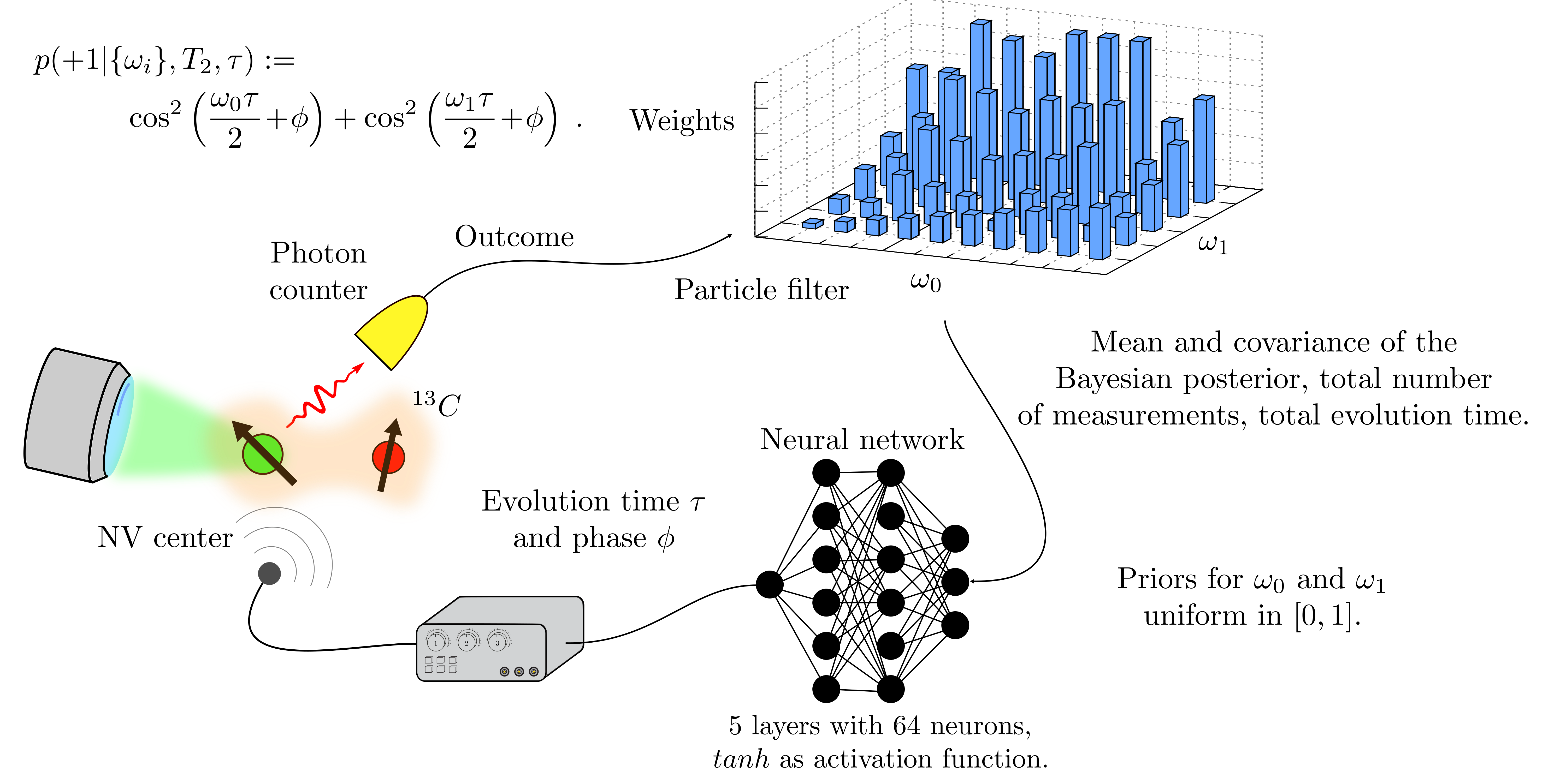
- main()
In the following we report the mean square error on the Bayesian estimators for the two frequencies for different strategies and different coherence times
. The resource is
either the total evolution time
or the number of measurements on the
NV center.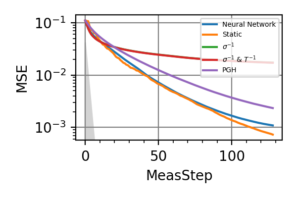
Fig. 23 invT2=0, Meas=128
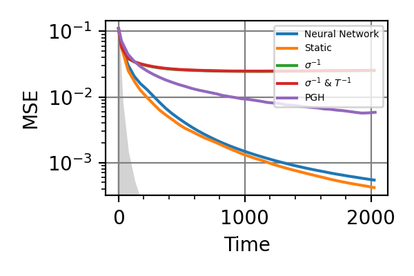
Fig. 24 invT2=0, Time=2048
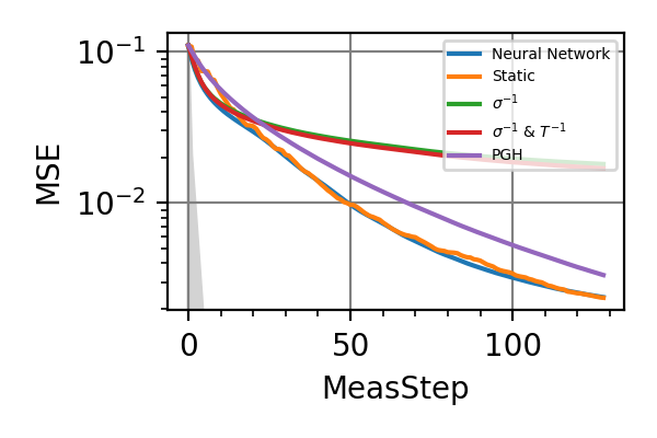
Fig. 25 invT2=0.01, Meas=128
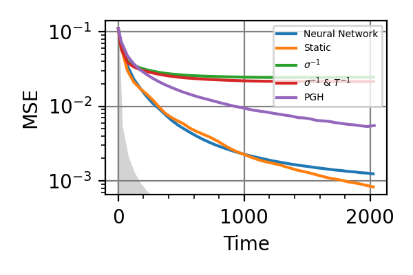
Fig. 26 invT2=0.01, Time=2048
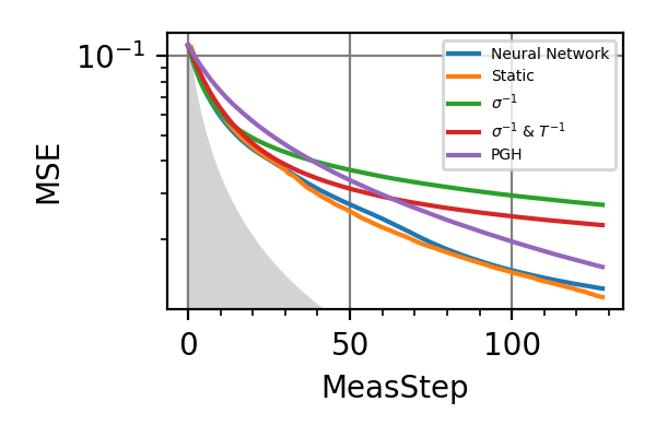
Fig. 27 invT2=0.1, Meas=128
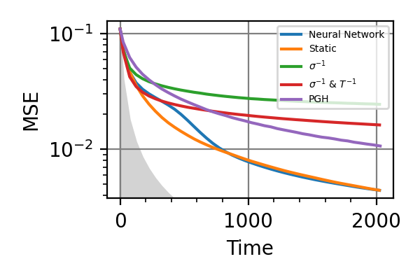
Fig. 28 invT2=0.1, Time=2048
The shaded grey areas in the above plot indicate the Bayesian Cramér-Rao bound, which is the the ultimate precision bound computed from the Fisher information.
From these simulations there seems to be no significant advantage in using an adaptive strategy for the simultaneous estimation of the two precession frequencies. Neither for large nor for small coherence times
.Notes
In a future work the alternative model of Eq.66 should be implemented. Being interested in the difference
, the sum of the frequencies
would be treated as a nuisance parameter.The absence on an advantage of the adaptive strategy over the non-adaptive one is probably also due to the hyper-simplified information passed to the neural network. We are in fact approximating a complex 2D posterior, with many peaks and valleys with a Gaussian. A better approach would be to train an autoencoder to compress the information contained in the posterior and pass it to the NN. The autoencoder will be trained to compress that class of distribution which are produced by the likelihood of the double precession frequency model.
All the simulations of this module have been done on a GPU NVIDIA GeForce RTX-4090-24GB.
- parse_args()
Arguments
- scratch_dir: str
Directory in which the intermediate models should be saved alongside the loss history.
- trained_models_dir: str = “./nv_center_double/trained_models”
Directory in which the finalized trained model should be saved.
- data_dir: str = “./nv_center_double/data”
Directory containing the csv files produced by the
performance_evaluation()and thestore_input_control()functions.- prec: str = “float32”
Floating point precision of the whole simulation.
- n: int = 64
Number of neurons per layer in the neural network.
- num_particles: int = 4096
Number of particles in the ensemble representing the posterior.
- iterations: int = 4096
Number of training steps.
NV center - Decoherence
- class DecoherenceSimulation(particle_filter: ParticleFilter, phys_model: NVCenterDecoherence, control_strategy: Callable, simpars: SimulationParameters, cov_weight_matrix: Optional[List] = None, random: bool = False, median: bool = False, loss_normalization: bool = False)
Bases:
StatelessMetrologyThis class does the same job of
StatelessMetrology, but it can append a randomly generated control time to the input_strategy Tensor produced by thegenerate_input()method and it can compute the median square error (MedianSE) instead of the mean square error (MSE) in theloss_function()method.Parameters passed to the constructor of the
DecoherenceSimulationclass.Parameters
- particle_filter:
ParticleFilter Particle filter responsible for the update of the Bayesian posterior on the parameters.
- phys_model:
NVCenterDecoherence Abstract description of the NC center for the characterization of the dephasing noise.
- control_strategy: Callable
Callable object (normally a function or a lambda function) that computes the values of the controls for the next measurement from the Tensor input_strategy, which is produced by the method
generate_input().- simpars:
SimulationParameters Contains the flags and parameters that regulate the stopping condition of the measurement loop and modify the loss function used in the training.
- cov_weight_matrix: List, optional
Positive semidefinite weight matrix. If this parameter is not passed then the default weight matrix is the identity, i.e.
.- random: bool = False
If this flag is True then a randomly chosen evolution time
 is added to the input_strategy
Tensor produced by
is added to the input_strategy
Tensor produced by generate_input().- median: bool = False
If this flag is True, then instead of computing the mean square error (MSE) from a batch of simulation the median square error (MedianSE) is computed. See the documentation of the
loss_function()method.Achtung! The median can be used in the training, however it means throwing away all the simulations in the batch except to the one that realizes the median. This is not an efficient use of the simulations in the training. When used the median should be always confined to the performances evaluation, while the training is to be carried out with the mean square error.
- loss_normalization: bool = False
If loss_normalization is True, then the loss is divided by the normalization factor
(67)
where
are the bounds
of the i-th parameter in phys_model.params
and are the diagonal entries of
cov_weight_matrix. is the total
elapsed evolution time, which can be different
for each estimation in the batch.Achtung! This flag should be used only if the resource is the total estimation time.
- generate_input(weights: Tensor, particles: Tensor, meas_step: Tensor, used_resources: Tensor, rangen: Generator)
This method returns the same input_strategy Tensor of the
generate_input()method, but, if the attribute random is True, an extra column is appended to this Tensor containing the randomly generated evolution time.
The value of  is
uniformly extracted in the interval
of the admissible values for the inverse of the
coherence time
is
uniformly extracted in the interval
of the admissible values for the inverse of the
coherence time  .
.
- loss_function(weights: Tensor, particles: Tensor, true_values: Tensor, used_resources: Tensor, meas_step: Tensor)
Computes the loss for each estimation in the batch.
If median is False, then it returns the same loss of the
loss_functionmethod, i.e. the square error for each simulation in the batch, called ,
where
,
where  runs from
  to ,
with the batchsize. If
the flag median is True, this method
returns the median square error of the batch,
in symbols
to ,
with the batchsize. If
the flag median is True, this method
returns the median square error of the batch,
in symbols
![\text{Median} [ \ell (\omega_k, \vec{\lambda})]](_images/math/9af250d4a22e9cb3e79fae7a8577e7d68e777e7b.svg) .
In order to compute it, the vector of
losses is
sorted, the element at position
.
In order to compute it, the vector of
losses is
sorted, the element at position
 is then the median of the losses in the batch.
Calling
is then the median of the losses in the batch.
Calling  the
position in the unsorted batch of the simulation
realizing the median, the outcome of this method
is the vector
the
position in the unsorted batch of the simulation
realizing the median, the outcome of this method
is the vector(68)
![\ell' (\omega_k, \vec{\lambda}) =
B \delta_{k, k_0} \text{Median}
[ \ell (\omega_k, \vec{\lambda})] \; .](_images/math/930087b1e14930617ba84bbf6708f37dc047fcf5.svg)
The advantage of using the median error is the reduced sensitivity to outliers with respect to the mean erro.
Achtung! Even if the performances evaluation can be performed with the median square error, the training should always minimize the mean square error.
- particle_filter:
- class NVCenterDecoherence(batchsize: int, params: List[Parameter], prec: Literal['float64', 'float32'] = 'float64', res: Literal['meas', 'time'] = 'meas')
Bases:
NVCenterModel describing an NV center subject to a variable amount of decoherence. The dephasing rate encodes some useful information about the environment, which can be recovered by estimating the transverse relaxation time and the decaying exponent.
Constructor of the
NVCenterDecoherenceclass.Parameters
- batchsize: int
Batchsize of the simulation, i.e. number of estimations executed simultaneously.
- params: List[
Parameter] List of unknown parameters to estimate in the NV center experiment, with their priors. It should contain the inverse of the characteristic time of the dephasing process, indicated with the symbol
and the exponent  of the decay. This last parameter carries
information on the spectral density
of the noise.
of the decay. This last parameter carries
information on the spectral density
of the noise.- prec{“float64”, “float32”}
Precision of the floating point operations in the simulation.
- res: {“meas”, “time”}
Resource type for the present metrological task. It can be either the total evolution time, i.e. time, or the total number of measurements on the NV center, i.e. meas.
- model(outcomes: Tensor, controls: Tensor, parameters: Tensor, meas_step: Tensor, num_systems: int = 1)
Model for the outcome of a photon counting measurement following a Ramsey sequence on the NV center sensor subject to dephasing noise. The probability of getting the outcome
is(69)

The evolution time
is controlled
by the trainable agent and and
are the two unknown characteristic parameters
of the noise. The factor 20 appearing
at the exponent is just the
normalization factor we used for .
- decoherence_estimation(args, batchsize: int, max_res: float, learning_rate: float = 0.001, gradient_accumulation: int = 1, cumulative_loss: bool = True, log_loss: bool = False, res: Literal['meas', 'time'] = 'meas', loss_normalization: bool = False, beta_nuisance: bool = False, fixed_beta: bool = False)
Simulates the Bayesian estimation of the decoherence parameters of a dephasing noise acting on an NV center. The control parameter is the free evolution time of the system during the Ramsey sequence. We have implement four strategies for the control of the evolution time:
Adaptive strategy with a trained neural network on the basis of the state of the particle filter (adaptive strategy).
Static strategy implemented with a neural network that receives in input the amount of already consumed resources (time or measurements)
Random strategy, with an evolution time chosen in the admissible interval for the values of
.Inverse time strategy. The evolution time is is
 for the measurement-limited
estimation and
for the measurement-limited
estimation and
 for the time-limited estimations,
where
for the time-limited estimations,
where  and
and
 .
These numerical coefficients come from
the optimization of the Fisher information.
For the simulations where is a nuisance
parameter
.
These numerical coefficients come from
the optimization of the Fisher information.
For the simulations where is a nuisance
parameter  is used also for the
time-limited estimation.
is used also for the
time-limited estimation.
This function trains the static and the adaptive strategies, and evaluates the error for all these four possibilities, in this order.
Achtung! In this example the static strategy is not implemented as a Tensor of controls for each individual measurement, like in the other examples. On the contrary it is implemented as a neural network that takes in input only the value of the consumed resources up to that point.
The measurement cycle is represented in the picture below.
Parameters
- args:
Arguments passed to the Python script.
- batchsize: int
Batchsize of the simulation, i.e. number of estimations executed simultaneously.
- max_res: float
Maximum amount of resources allowed to be consumed in the estimation.
- learning_rate: float = 1e-3
Initial learning rate for the neural networks, for both the adaptive and static strategies. The learning rate decays with
InverseSqrtDecay.- gradient_accumulation: int = 1
Flag of the
train()function.- cumulative_loss: bool = False
Flag
cumulative_loss.- log_loss: bool = False
Flag
log_loss.- res: {“meas”, “time”}
Type of resource for the simulation. It can be either the number of measurements or the total evolution time.
- loss_normalization: bool = False
Parameter loss_normalization passed to the constructor of the
NVCenterDecoherenceclass.- beta_nuisance: bool = False
If this flag is True, the loss is computed only from the error on the inverse decay time
.- fixed_beta: bool = False
If this flag is True the decay exponent is set to
 .
.
- main()
In this example we characterize the dephasing process of an NV center. We study three cases. In the first one the decaying exponent
is unknown and it is treated as
a nuisance parameter. Therefore, only the
precision on the inverse decay time appears
in the loss (the MSE). In the second case
is known and fixed
( ), and only
is estimated. In the third case
both and
are unknown and are parameters of interest,
but their MSE are not evenly weighted:
the error
), and only
is estimated. In the third case
both and
are unknown and are parameters of interest,
but their MSE are not evenly weighted:
the error  weights
half of
weights
half of  . This
is done t equilibrate the different priors on
the parameters and consider them on an equal
footage.
. This
is done t equilibrate the different priors on
the parameters and consider them on an equal
footage.The prior on
is uniform
in (0.01, 0.1), and that of
is uniform in (0.075, 0.2) (when it is not
fixed), so that the interval
for the actual exponent, which is  (see
(see model()) is (1.5, 4) 5.In the following we report the estimator error (MSE) for a bounded number of measurement (on the left), and for a bounded total evolution time (on the right). These simulations are done by calling the function
decoherence_estimation().The adaptive and static strategies are compared with two simple choices for the controls. The first is a randomize strategy, according to which the inverse of the evolution time is randomly selected uniformly in (0.01, 0.1), while the second is a
 strategy, according to which the
inverse of the evolution time is chosen to be the current
estimator for the inverse of the coherence time.
strategy, according to which the
inverse of the evolution time is chosen to be the current
estimator for the inverse of the coherence time.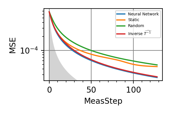
Fig. 29 Meas=128, beta nuisance
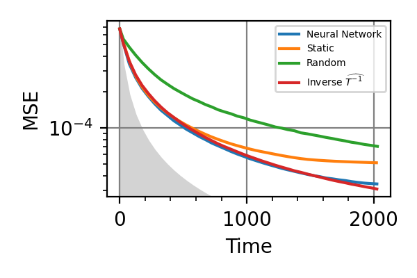
Fig. 30 Time=2048, beta nuisance
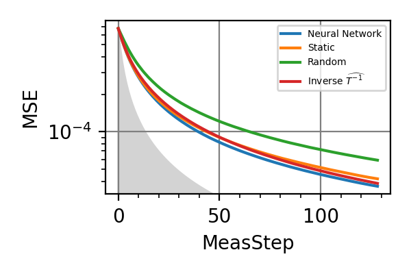
Fig. 31 Meas=128, fixed beta
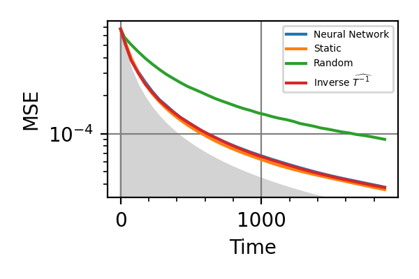
Fig. 32 Time=2048, fixed beta
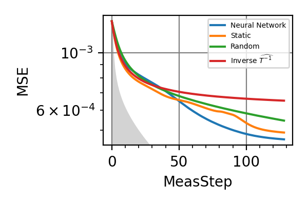
Fig. 33 Meas=128, both parameters
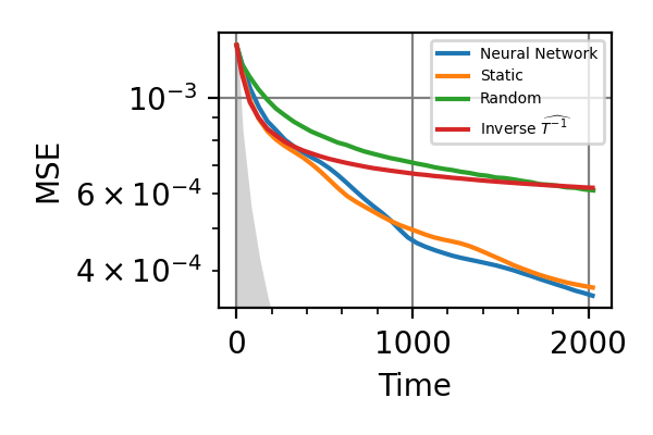
Fig. 34 Time=2048, both parameters
The shaded grey areas in the above plot indicate the Bayesian Cramér-Rao bound, which is the the ultimate precision bound computed from the Fisher information.
There is no advantage in using a NN instead of the strategies that optimize the Fisher information.
Notes
Some application of the estimation of the decoherence time involve the measure of the radical concentration in a biological sample and the measurement of the local conductivity through the Johnson noise.
All the training of this module have been done on a GPU NVIDIA Tesla V100-SXM2-32GB, each requiring
hours.
- parse_args()
Arguments
- scratch_dir: str, required
Directory in which the intermediate models should be saved alongside the loss history.
- trained_models_dir: str = “./nv_center_decoherence/trained_models”
Directory in which the finalized trained model should be saved.
- data_dir: str = “./nv_center_decoherence/data”
Directory containing the csv files produced by the
performance_evaluation()and thestore_input_control()functions.- prec: str = “float32”
Floating point precision of the whole simulation.
- n: int = 64
Number of neurons per layer in the neural network.
- num_particles: int = 2048
Number of particles in the ensemble representing the posterior.
- iterations: int = 4096
Number of training steps.
- scatter_points: int = 32
Number of points in the Resources/Precision csv produced by
performance_evaluation().
Dolinar (Dolan) receiver
- class AgnosticDolinar(batchsize: int, params: List[Parameter], n: int, resources: str = 'alpha', prec: str = 'float64')
Bases:
StatefulPhysicalModelSchematization of the agnostic Dolinar receiver 6.
The task is to discriminate between
 and
and  , given a single copy
of
, given a single copy
of  and
and  copies
of
copies
of  , that have been
prepared in another lab. At difference with the
usual Dolinar receiver the intensity
of the signal
, that have been
prepared in another lab. At difference with the
usual Dolinar receiver the intensity
of the signal  is not known, but can
be estimated from
is not known, but can
be estimated from  to adapt the strategy. The physical motivations
behind this model is that of a series of wires,
with only one carrying the signal, subject
to a loss noise of fluctuating intensity.
to adapt the strategy. The physical motivations
behind this model is that of a series of wires,
with only one carrying the signal, subject
to a loss noise of fluctuating intensity.- 6
F. Zoratti, N. Dalla Pozza, M. Fanizza, and V. Giovannetti, Phys. Rev. A 104, 042606 (2021).
Constructor of the
AgnosticDolinarclass.Parameters
- batchsize: int
Number of agnostic Dolinar receivers simulated at the same time in a mini-batch.
- params: List[
Parameter] List of parameters. It must contain the continuous parameter alpha with its admissible range of values, and the discrete sign parameter, that can take the values (-1, +1).
- n: int
Number of states
 that the
agnostic Dolinar receiver consumes to make a
decision on the sign of the sign of the signal.
that the
agnostic Dolinar receiver consumes to make a
decision on the sign of the sign of the signal.Achtung! Note that in the simulation n+1 measurement are actually performed, because both outputs of the last beam splitter are measured.
- resources: {“alpha”, “step”}
Resources of the model, can be the amplitude
of the signal or the number
of state consumed
in the procedure.- prec: str = “float64”
Floating point precision of the model.
- count_resources(resources: Tensor, outcomes: Tensor, controls: Tensor, true_values: Tensor, state: Tensor, meas_step: Tensor) Tensor
The resources can be either the number of states
consumed,
which is update after every beam splitter,
or the amplitude , that is
related to the mean number of photons in
the signal.
- initialize_state(parameters: Tensor, num_systems: int) Tensor
State initialization for the agnostic Dolinar receiver. The state contains the amplitude of the remaining signal after the measurements (for both hypothesis) and the total number of measured photons.
- model(outcomes: Tensor, controls: Tensor, parameters: Tensor, state: Tensor, meas_step: Tensor, num_systems: int = 1)
Probability of observing the number of photons outcomes in a photon counter measurement in the agnostic Dolinar receiver.
- perform_measurement(controls: Tensor, parameters: Tensor, true_state: Tensor, meas_step: Tensor, rangen: Generator)
The signal
and
the reference states are
sequentially mixed on a beam splitter
with tunable transmission  , and
one output of the beam splitter is measured
through photon counting, while the other gets
mixed again. The left over signal after
n uses of the beam splitter is then
measured on a photon counter.
, and
one output of the beam splitter is measured
through photon counting, while the other gets
mixed again. The left over signal after
n uses of the beam splitter is then
measured on a photon counter.
- class DolinarSimulation(particle_filter: ParticleFilter, phys_model: AgnosticDolinar, control_strategy: Callable, simpars: SimulationParameters, loss: int = 3)
Bases:
StatefulSimulationSimulation class for the agnostic Dolinar receiver. It works with a
ParticleFilterand aAgnosticDolinarobjects.The measurement loop is showed in the following picture.
Constructor of the
DolinarSimulationclass.Parameters
- particle_filter:
ParticleFilter Particle filter responsible for the update of the Bayesian posterior on
and on the sign of the signal. It
contains the methods for applying the Bayes
rule and computing Bayesian estimators
from the posterior.- phys_model:
AgnosticDolinar Model of the agnostic Dolinar receiver.
- simpars:
SimulationParameters Parameter simpars passed to the class constructor.
- loss: int = 3
Type of loss to be used in the simulation. It regulates the behavior of the
loss_function()method. There are nine possible losses to choose from. These are explained in the documentation ofloss_function().
- generate_input(weights: Tensor, particles: Tensor, state_ensemble: Tensor, meas_step: Tensor, used_resources: Tensor, rangen: Generator)
This method collects the information on
and on the sign of the signal
produced by the particle filter and builds from
them the input_strategy object to be fed
to the neural network. This Tensor has nine
scalar components, that are: , the normalized
intensity of the signal after the
measurements, assuming that it was
at the beginning.
, the normalized
intensity of the signal after the
measurements, assuming that it was
at the beginning. , the mean posterior
estimator for signal intensity assuming
.
, the mean posterior
estimator for signal intensity assuming
. , the variance of the
posterior distribution for the signal intensity,
assuming .
, the variance of the
posterior distribution for the signal intensity,
assuming . , the normalized
intensity of the signal after the
measurements, assuming that it was
at the beginning.
, the normalized
intensity of the signal after the
measurements, assuming that it was
at the beginning. , the mean posterior
estimator for signal intensity assuming
.
, the mean posterior
estimator for signal intensity assuming
. , the variance of the
posterior distribution for the signal intensity,
assuming .
, the variance of the
posterior distribution for the signal intensity,
assuming . the posterior probability
for the original signal to be ,
the posterior probability
for the original signal to be ,the index of the current measurement meas_step normalized against the total number of measurements,
the total number of photons measured, up to the point this method is called.
- loss_function(weights: Tensor, particles: Tensor, true_state: Tensor, state_ensemble: Tensor, true_values: Tensor, used_resources: Tensor, meas_step: Tensor)
The loss of the agnostic Dolinar receiver measures the error in guessing the sign of the signal
 , after the signal
has been completely measured.
, after the signal
has been completely measured.There are nine possible choices for the loss, which can be tuned through the parameter loss passed to the constructor of the
DolinarSimulationclass. Before analyzing one by one these losses we establish some notation. is the posterior
probability that the original signal is
 ,
,
 ,
,  is the sign of the signal in
  ,
and
,
and  is the total number of observed
photons. The error probability given by the resource
limited Helstrom bound is
indicated with
is the total number of observed
photons. The error probability given by the resource
limited Helstrom bound is
indicated with  . This is computed
by the function
. This is computed
by the function helstrom_bound(). We also define the Kronecker delta function(70)

There are two possible policies for guessing the signal sign, that we indicate respectively with
 and
and  .
They are respectively
.
They are respectively(71)

and
(72)

The possible choices for the loss are
loss=0:
 ,
,loss=1:
 ,
,loss=2:
 ,
,loss=3:
 ,
,loss=4:
 ,
,loss=5:
 ,
,loss=6:
 ,
,loss=7:
 ,
,loss=8:
 ,
,
Notes
The optimization with loss=3 works better for small
then for large .
This is because the scalar loss is the mean
of the error probability on the batch and it
is not so relevant to optimize the estimations
those regions
of the parameter that have low
error probability anyway. To summarize, loss=3
makes the optimization concentrate on the region of small
, since this region dominates the error.Achtung!: A constant added to the loss is not irrelevant for the training, since the loss itself and not only the gradient is appears in the gradient descent update.
- particle_filter:
- dolinar_receiver(args, num_steps: int, loss: int = 3, learning_rate: float = 0.01)
Training and performance evaluation of the neural network and the static strategies that control the beam splitter reflectivity in the agnostic Dolinar receiver.
Parameters
- args:
Arguments passed to the Python script.
- num_steps: int
Number of reference states
in the Dolinar receiver.- loss: int = 3
Type of loss used for the training, among the ones described in the documentation of
loss_function(). The loss used for the performances evaluation is always loss=0.- learning_rate: float = 1e-2
Initial learning rate for the neural network. The initial learning rate of the static strategy is fixed to 1e-2. They both decay with
InverseSqrtDecay.
- helstrom_bound(batchsize: int, n: int, alpha: Tensor, iterations: int = 200, prec: str = 'float64')
Calculates the Helstrom bound for the agnostic Dolinar receiver with n copies of
. It is the lower bound
on the error probability for the
discrimination task and it is given by the
formula(73)

where
 is the probability
distribution of a Poissonian variable, i.e.
is the probability
distribution of a Poissonian variable, i.e.(74)

Parameters
- batchsize: int
Number of bounds to be computed simultaneously, it is the first dimension of the alpha Tensor.
- n: int
Number of copies of
at disposal.- alpha: Tensor
Tensor of shape (batchsize, 1), with the amplitudes of the coherent states for each discrimination task.
- iterations: int = 200
There is no closed formula for the error probability, this parameter is the number of summand to be computed in Eq.73.
- prec: str = “float64”
Floating point precision of the alpha parameter.
Returns
- Tensor:
Tensor of shape (batchsize, 1) and type prec containing the evaluated values of the Helstrom error probability for the discrimination taks.
- main()
We have trained the optimal adaptive and static strategies for the agnostic Dolinar receiver.
The error probabilities as a function of
are reported in the following
figure for  and
and  reference states
, for two different
training losses (loss=3 and loss=6).
reference states
, for two different
training losses (loss=3 and loss=6).The Heterodyne and Photon counting are two 2-stage adaptive strategies based on first measuring all the reference state
and then trying to discriminate the signal based
on the acquired information 5.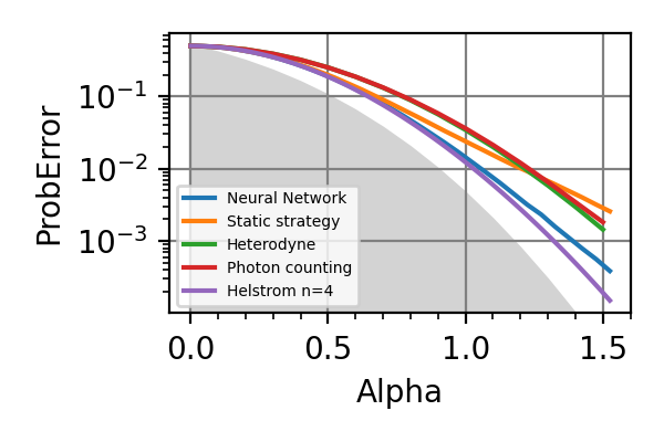
Fig. 35 n=4, loss=3
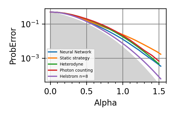
Fig. 36 n=8, loss=3
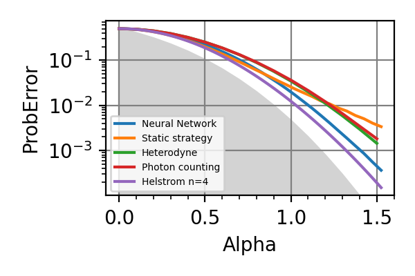
Fig. 37 n=4, loss=6
Fig. 38 n=8, loss=6
The shaded grey areas in the above plot indicate the Helstrom bound for the discrimination of
.The loss=3 seems to be uniformly superior to loss=6 for every value of
.
The advantage of using the neural network strategy
is very contained with respect to already known
strategies for but it is significant
for . Instead of a NN a decision tree
could have also been a viable strategy for controlling
the beam splitters as done in the module
dolinar_three. As expected the gap between the precision of the adaptive and of the non-adaptive strategies increases with the number of photons in the signal.Notes
The loss used in calling
performance_evaluation()is always loss=0.The resources used in calling
store_input_control()are always the number of measurements.An application of machine learning (decision trees) to the Dolinar receiver have been presented also by Cui et al 7.
Known bugs: the training on the GPU freezes if the parameter alpha_bound is set to be too large. This is probably due to a bug in the implementation of the function random.poisson. A preliminary work-around has shown that reimplementing the extraction from a Poissonian distribution with random.categorical would solve the problem.
All the training of this module have been done on a GPU NVIDIA Tesla V100-SXM2-32GB, each requiring
hours.- 7
C. Cui, W. Horrocks, S. Hao et al., Light Sci Appl. 11, 344 (2022).
- parse_args()
Arguments
- scratch_dir: str
Directory in which the intermediate models should be saved alongside the loss history.
- trained_models_dir: str = “./dolinar/trained_models”
Directory in which the finalized trained model should be saved.
- data_dir: str = “./dolinar/data”
Directory containing the csv files produced by the
performance_evaluation()and thestore_input_control()functions.- prec: str = “float64”
Floating point precision of the whole simulation.
- batchsize: int = 4096
Batchsize of the simulation.
- n: int = 64
Number of neurons per layer in the neural network.
- num_particles: int = 512
Number of particles in the ensemble representing the posterior.
- num_steps: int = 8
Number of reference states
,
i.e. number of beam splitters.- training_loss: int = 3
Loss used in the training. It is an integer in th range [0, 8]. The various possible losses are reported in the description of the
loss_function()method.- iterations: int = 32768
Number of training steps.
Quantum ML classifier
- class CoherentStates(batchsize: int, prec: str = 'float64')
Bases:
objectThis class contains the methods to operated on one ore more bosonic wires carrying coherent states. It can’t deal with squeezing or with noise, only with displacements, phase shifts and photon counting measurements.
Notes
The covariance matrix of the system is always proportional to the identity and corresponds to zero temperature.
Constructor of the
CoherentStatesclass.Parameters
- batchsize: int
Number of experiments that are simultaneously treated by the object.
Achtung! This is not the number of bosonic lines that an object of this class can deal with. This is in fact not an attribute of the class, and is not fixed during the initialization.
- apply_bs_network(variables_real: Tensor, variables_imag: Tensor, input_channels: Tensor, num_wires: int)
Applies the beam splitter network identified by variables_real and variables_imag to the state carried by the bosonic lines.
Parameters
- variables_real: Tensor
Tensor of shape (batchsize, ?, num_wires, num_wires) and type prec.
- variables_imag: Tensor
Tensor of shape (batchsize, ?, num_wires, num_wires) and type prec.
- input_channels: Tensor
Displacement vector of the bosonic wires. It is a Tensor of type prec and shape (batchsize, ?, 2 num_wires). The components of the i-th wire are at position i and i+num_wires.
- num_wires: int
Number of wires in the system.
Returns
- Tensor
Tensor of shape (batchsize, ?, 2 num_wires) and type prec, containing the evolved displacements of the bosonic wires state.
- apply_bs_network_from_unitary(unitary: Tensor, input_channels: Tensor)
Applies the beam splitter identified by variables_real and variables_imag.
Parameters
- unitary: Tensor
Tensor of shape (batchsize, ?, num_wires, num_wires) and type complex64 if prec is float32 or complex128 if prec if float64.
- input_channels: Tensor
Displacement vector of the bosonic wires. It is a Tensor of type prec and shape (batchsize, ?, 2 num_wires). The components of the i-th wire are at position i and i+num_wires.
Returns
- Tensor
Tensor of shape (batchsize, ?, 2 num_wires) and type prec, containing the evolved displacements of the bosonic wires wires.
Notes
The covariance matrix of the system is always proportional to the identity and corresponds to zero temperature.
- beamsplitter(input1: Tensor, input2: Tensor, theta: Tensor, phi: Tensor) Tuple[Tensor, Tensor]
Beam splitter (BS) operating on two bosonic modes carrying coherent states. It returns the two states outputted by the BS.
Parameters
- input1: Tensor
Tensor of shape (bs, ?, 2) and of type prec containing the x and y components of the first incident state on the BS.
- input2: Tensor
Tensor of shape (bs, ?, 2) and of type prec containing the x and y components of the second incident state on the BS.
- theta: Tensor
Tensor of shape (bs, ?) and of type prec. It contains the transmission coefficient of the BS. It is indicated with
in the formulas.- phi:
Tensor of shape (bs, ?) and of type prec. It contains the phase applied by the BS. It is indicated with
in the formulas.
Returns
- Tensor:
Tensor of shape (bs, ?, 2) and type prec. Contains the first output state of the BS.
- Tensor:
Tensor of shape (bs, ?, 2) and type prec. Contains the second output state of the BS.
- mean_phot(input_state: Tensor) Tensor
Returns the mean photon number on a coherent state.
Parameters
- input_state: Tensor
Tensor of shape (bs, ?, 2) and of type prec containing the x and y components of the coherent state.
Returns
- Tensor
Tensor of shape (bs, ?) and type prec containing the average number of photons of the coherent states described in input_state.
- phase_shift(input_state: Tensor, phase: Tensor) Tensor
Applies a phase shift on the coherent states encoded in input_state.
Parameters
- input_state: Tensor
Tensor of shape (bs, ?, 2) and of type prec containing the x and y components of the coherent state to be rotated.
- phase: Tensor
Tensor of shape (bs, ?) containing the phase for the rotation of each state in the batch.
Returns
- Tensor:
Tensor of shape (bs, ?, 2) and of type prec containing the rotated coherent state.
- photon_counter(input_state: Tensor, rangen: Generator, num_systems: int = 1) Tuple[Tensor, Tensor]
Photon counting measurement on a bosonic line carrying a coherent state.
Parameters
- input_state: Tensor
Tensor of shape (bs, ?, 2) and of type prec containing the x and y components of the coherent state on which the photon counting measurement will be performed.
- rangen: Generator
Random number generator from the module
tensorflow.random.- num_systems: int = 1
Number of independent coherent states processed per batch. It is the size of the second dimension of input_state.
Returns
- outcomes: Tensor
Tensor of shape (bs, num_systems, 1) and type prec containing the outcomes of the photon counting measurement (the number of photons).
- log_prob: Tensor
Tensor of shape (bs, num_systems) and type prec containing the logarithm of the probability of the observed number of photons.
- postselect_photon_counter(input_state: Tensor, outcomes: Tensor) Tensor
Returns the logarithm of the probability of observing outcomes after a photon counting measurement on input_state.
Parameters
- input_state: Tensor
Tensor of shape (bs, ?, 2) and of type prec containing the x and y components of the coherent state on which the photon counting measurement is performed.
- outcomes: Tensor
Tensor of shape (bs, ?, 1) and type prec containing the outcomes of the photon counting measurement (the number of photons).
Returns
- log_prob: Tensor
Tensor of shape (bs, ?) and type prec containing the logarithm of the probability of observing outcomes on input_state.
- class QMLDiscriminator(batchsize: int, params: List[Parameter], num_ref: int, resources: str = 'alpha', arch: str = 'serial', decision_tree: bool = False, prec: str = 'float64')
Bases:
StatefulPhysicalModel,CoherentStatesBlueprint class for the quantum Machine Learning (QML) based classifier able to distinguish between three coherent states
 ,
,
 ,
,  ,
given copies of each of them, which
constitute the quantum training set.
The signal state is a single copy of a
coherent state, promised to be one of the
three training states, i.e.
,
given copies of each of them, which
constitute the quantum training set.
The signal state is a single copy of a
coherent state, promised to be one of the
three training states, i.e.  with s=0, 1, 2.
Notes
The priors on the real components of the training states
,
,
are uniform, as the prior on the signal classes
s=0, 1, 2.Attributes
- bs: int
The batchsize of the physical model, i.e., the number of simultaneous signal testings simulated.
- controls: List[
Control] The controls of the QML classifier are the transmission coefficient and the extra phase of the beam splitter that precedes the photon counting. These can be chosen adaptively according to the previous measurements outcomes.
- params: List[
Parameter] List of parameters to be estimated, passed to the class constructor. These are the real components of the unknown training states (continuous parameter), and the class of the signal.
- controls_size: int = 2
Number of scalar controls in the QML classifier, i.e. 2, the two angles
and characterizing the beam splitter
transformation performed by
beamsplitter().- d: int = 7
The number of unknown parameters to estimate, i.e. 7.
- state_specifics:
StateSpecifics Size of the state of the apparatus, which can be 2 for the serial architecture or 6 for the parallel, plus the type of the state, i.e. prec. If decision_tree=True the size of the state is increased by one.
- recompute_state: bool = True
Flag to the constructor of the
PhysicalModelclass.- outcomes_size: int = 1
Number of scalar outcomes for each measurement in the apparatus, i.e. one, the number of photons in the photon counter.
- prec: str
The floating point precision of the controls, outcomes, and parameters.
- num_ref: int
Number of copies of each training state, passed to the class constructor.
- num_steps: int
Total number of photon counting measurements in the apparatus. It depends on num_ref and on the architecture, in particular it is 3 num_ref+1 for the serial apparatus and 3 num_ref+3 for the parallel one.
- resources: {“alpha”, “step”}
Resource type passes to the class constructor. It can be the average number of photons in the device (“alpha”) or the number of measurements (“step”).
- dt: bool
Flag decision_tree passed to the class constructor. It should be activated if a decision tree is used for controlling the beam splitters.
- arch: {“serial”, “parallel”}
Architecture of the QML classifier passed to the class constructor. An object of the child class
QMLDiscriminatorSerialwill have arch=”serial”, while an instance ofQMLDiscriminatorParallelwill have arch=”parallel”.
Constructor of the
QMLDiscriminatorclass.Parameters
- batchsize: int
Batchsize of the physical model, i.e., the number of simultaneous estimations.
- params: List[
Parameter] A list of unknown parameters to be estimated, alongside the corresponding sets of admissible values. For the three states Dolinar these are the x and y components of
,
,
(six continuous parameters in total) plus the
class of the signal, which is a discrete parameter
that takes values in the set {0, 1, 2}.- num_ref: int
Number of copies of each training state.
- resources: {“alpha”, “step”}
Two types of resource counting are possible in the apparatus. The first is the the total number of photon counting measurements, corresponding to the value “step” for the resources parameter. The second is the mean number of photons in the apparatus, corresponding to the value “alpha” for this parameter. The average photon number is
(75)

where
is the number of training copies,
i.e. num_ref.- arch: {“serial”, “parallel”}
Architecture of the QML classifier.
- decision_tree: bool = False
If this flag is True, then the physical model of the device is set up to be used with a decision tree controlling the beam splitters. This affect the state size, which now contains an integer that univocally identifies the string of outcomes that have already appeared in the photon counting measurements.
- prec: str = “float64”
Floating point precision of the controls, outcomes, and parameters.
- count_resources(resources: Tensor, outcomes: Tensor, controls: Tensor, true_values: Tensor, state: Tensor, meas_step: Tensor) Tensor
The resources can be either the number of measurement steps or the mean number of photons in the system. In the second case the resource is considered consumed after the last photon counting measurement closing the device.
- class QMLDiscriminatorParallel(batchsize: int, params: List[Parameter], num_ref: int, resources: str = 'alpha', decision_tree: bool = False, prec: str = 'float64')
Bases:
QMLDiscriminatorParallel strategy for classifying a coherent state, given three hypothesis.
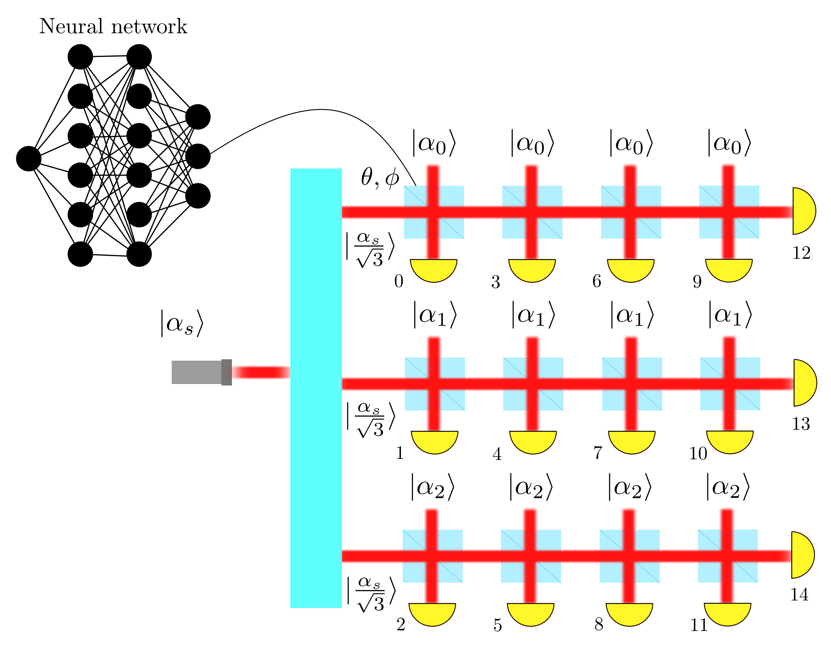
The original signal is first equally splitted on three wires, i.e.
 . On each
line the signal is mixed with the copies of the same
training state.
. On each
line the signal is mixed with the copies of the same
training state.The order of the measurements is show in the figure near the symbol for the photon counter. The measurements are not really done in parallel as it can be seen. All the outcomes of the previous photon counters contributes to the determination of the next controls through the particle filter and the neural network (or the decision tree). In order to realize the measurements in this order the optical path along the the wires should be prolonged differently.
Constructor of the
QMLDiscriminatorParallelclass.Parameters
- batchsize: int
Number of simultaneous estimations.
- params: List[
Parameter] Contains the real components of the unknown training states and the signal to be classified.
- num_ref: int
Number of training states for each class.
- resources: {“alpha”, “step”}
Type of resources counted.
- decision_tree: bool = False
Indicates that a decision tree is used for controlling the beam splitters.
- prec:
Floating point precision of the estimation.
- initialize_state(parameters: Tensor, num_systems: int) Tensor
Initializes the true state of the signal
 for the parallel device.
Parameters
- parameters: Tensor
Tensor of shape (bs, num_system, 7) and type prec containing the real components of the three training states and the index classifying the true signal (the seventh parameter).
- num_systems: int
Size of the second dimension of the parameters Tensor. It is the number of systems treated per batch element.
Returns
- Tensor:
Tensor of shape (bs, num_system, 6) containing the state of the true signal, equally distributed on the three lines of the discrimination device with parallel architecture. If decision_tree=True the size of the last dimension of the returned Tensor is 7.
- model(outcomes: Tensor, controls: Tensor, parameters: Tensor, state: Tensor, meas_step: Tensor, num_systems: int = 1)
Probability of observing a certain number of photons in a photon counting measurement in the parallel device.
Parameters
- outcomes:
Tensor of shape (bs, num_systems, 1) and type prec containing the observed number of photons in a measurement.
- controls: Tensor
Tensor of shape (bs, num_systems, 2) and of type prec containing the two angles
and
characterizing the BS placed
before a photon counter.- parameters: Tensor
Tensor of shape (bs, num_systems, 7) and type prec containing the six real components of the three training states plus the signal class.
- state: Tensor
Tensor of shape (bs, num_systems, 6) containing the real components in the phase space of the signal traveling through the three wires of the apparatus. If decision_tree=True the shape of this Tensor is (bs, num_systems, 7) and it contains also the whole history of outcomes codified in the last entry.
- meas_step: Tensor
Tensor of shape (bs, num_systems, 1) and type prec. It is the index of the current measurement and starts from zero.
- num_systems: int = 1
Number of system treated for each element of the batch.
Return
- log_prob: Tensor
Tensor of shape (bs, num_systems) and type prec containing the logarithm of the probability of getting the observed number of photons.
- state: Tensor
Tensor of shape (bs, num_systems, 6) and type prec with the state of the signal evolved after the photon counting measurement. If decision_tree=True the shape of this Tensor is (bs, num_systems, 7) and it contains also the whole history of outcomes codified in the last entry.
- perform_measurement(controls: Tensor, parameters: Tensor, true_state: Tensor, meas_step: Tensor, rangen: Tensor)
Mixing of the signal on one wire with the corresponding training state and photon counting on one end of the beam splitter.
Parameters
- controls: Tensor
Tensor of shape (bs, 1, 2) and of type prec containing the two angles
and
characterizing the BS placed
before a photon counter.- parameters: Tensor
Tensor of shape (bs, 1, 7) and type prec containing the six real components of the three training states plus the signal class.
- true_state: Tensor
Tensor of shape (bs, 1, 6) containing the real components in the phase space of the signal traveling through the three wires of the apparatus. If decision_tree=True the shape of this Tensor is (bs, 1, 7) and it contains also the whole history of outcomes codified in the last entry.
- meas_step: Tensor
Tensor of shape (bs, 1, 1) and type prec. It is the index of the current measurement and starts from zero.
Return
- outcomes: Tensor
Tensor of shape (bs, 1, 1) and type prec containing the number of photons observed in the photon counting measurement.
- log_prob: Tensor
Tensor of shape (bs, 1) and type prec containing the logarithm of the probability of getting the observed number of photons.
- state: Tensor
Tensor of shape (bs, 1, 6) and type prec with the state of the signal evolved after the photon counting measurement. If decision_tree=True the shape of this Tensor is (bs, 1, 7) and it contains also the whole history of outcomes codified in the last entry.
- class QMLDiscriminatorSerial(batchsize: int, params: List[Parameter], num_ref: int, resources: str = 'alpha', prec: str = 'float64', decision_tree: bool = False)
Bases:
QMLDiscriminatorSerial strategy for classifying a coherent state, given three hypothesis.
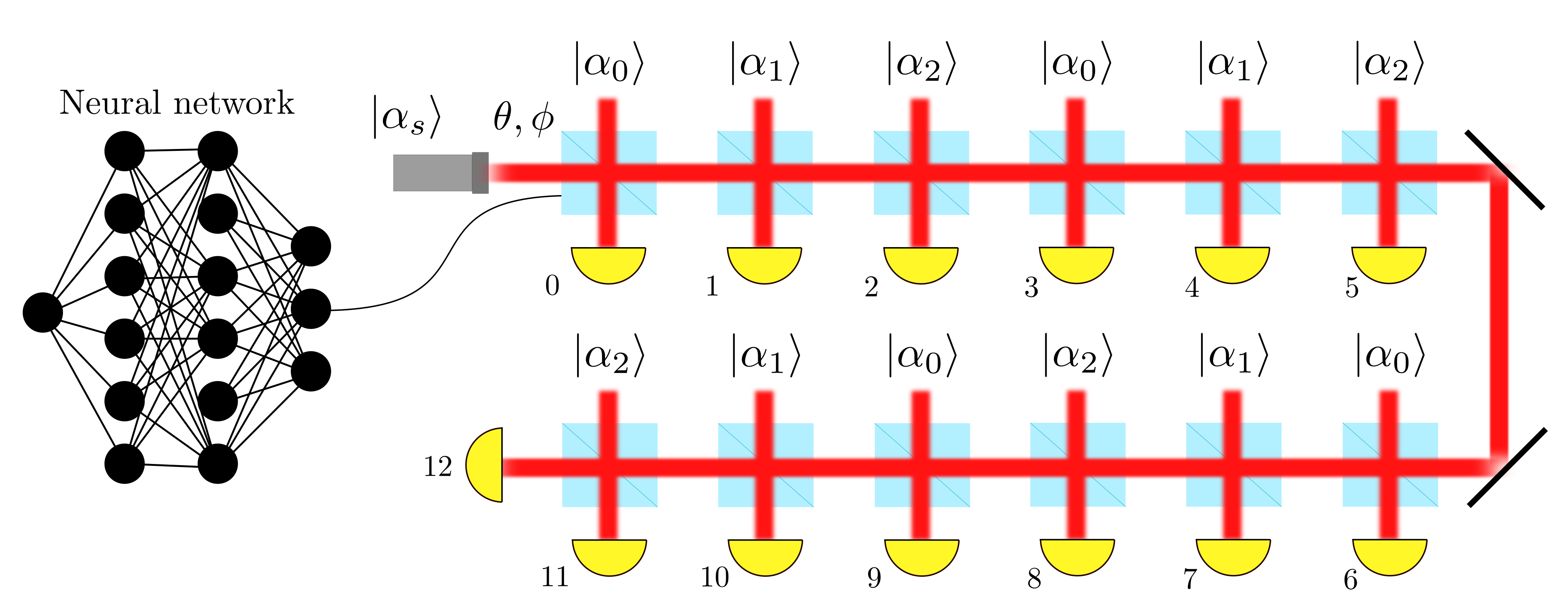
The signal
is alternatively
mixed with the training states and measured.The order of the measurements is shown in the figure near the symbols for the for the photon counters. All the outcomes of the previous photon counters contribute to the determination of the next controls through the particle filter and the neural network (or the decision tree)
Constructor of the
QMLDiscriminatorSerialclass.Parameters
- batchsize: int
Number of simultaneous estimations.
- params:
Real components of the unknown training states and signal to be classified.
- num_ref: int
Number of training states for each class.
- resources: {“alpha”, “step”}
Type of resources counted.
- prec:
Floating point precision of the estimation.
- initialize_state(parameters: Tensor, num_systems: int) Tensor
Initializes the true state of the signal
for the serial architecture.Parameters
- parameters: Tensor[bs, num_systems, 7]
Tensor of shape (bs, num_system, 7) and type prec containing the real components of the three training states and the index classifying the true signal (the seventh parameter).
- num_systems: int
Size of the second dimension of the parameters tensor. It is the number of systems treated per batch element.
Returns
- Tensor:
Tensor of shape (bs, num_system, 2) containing the initial state of the signal
, computed according
to parameters. If decision_tree=True the size of the
last dimension of the returned Tensor is 3.
- model(outcomes: Tensor, controls: Tensor, parameters: Tensor, state: Tensor, meas_step: Tensor, num_systems: int = 1) Tuple[Tensor, Tensor]
Probability of observing a certain number of photons in a photon counting measurement in the serial device.
Parameters
- outcomes:
Tensor of shape (bs, num_systems, 1) and type prec containing the observed number of photons in a measurement.
- controls: Tensor
Tensor of shape (bs, num_systems, 2) and of type prec containing the two angles
and
characterizing the BS placed before
a photon counter.- parameters: Tensor
Tensor of shape (bs, num_systems, 7) and type prec containing the six real components of the three training states plus the signal class.
- state: Tensor
Tensor of shape (bs, num_systems, 2) containing the real components in the phase space of the signal traveling through the apparatus. If decision_tree=True the shape of this Tensor is (bs, num_systems, 3) and it contains also the whole history of outcomes codified in the last entry.
- meas_step: Tensor
Tensor of shape (bs, num_systems, 1) and type prec. It is the index of the current measurement and starts from zero.
- num_systems: int = 1
Number of system treated for each element of the batch.
Return
- log_prob: Tensor
Tensor of shape (bs, num_systems) and type prec containing the logarithm of the probability of getting the observed number of photons.
- state: Tensor
Tensor of shape (bs, num_systems, 2) and type prec with the state of the signal evolved after the photon counting measurement. If decision_tree=True the shape of this Tensor is (bs, num_systems, 3) and it contains also the whole history of outcomes codified in the last entry.
- perform_measurement(controls: Tensor, parameters: Tensor, true_state: Tensor, meas_step: Tensor, rangen: Tensor) Tuple[Tensor, Tensor, Tensor]
Mixing of the signal with the training state and photon counting on one end of the beam splitter.
Parameters
- controls: Tensor
Tensor of shape (bs, 1, 2) and of type prec containing the two angles
and
characterizing the BS placed
before a photon counter.- parameters: Tensor
Tensor of shape (bs, 1, 7) and type prec containing the six real components of the three training states plus the signal class.
- true_state: Tensor
Tensor of shape (bs, 1, 2) containing the real components in the phase space of the signal traveling through the apparatus. If decision_tree=True the shape of this Tensor is (bs, 1, 3) and it contains also the whole history of outcomes codified in the last entry.
- meas_step: Tensor
Tensor of shape (bs, 1, 1) and type prec. It is the index of the current measurement and starts from zero.
- rangen: Generator
Random number generator from the module
tensorflow.random.
Return
- outcomes: Tensor
Tensor of shape (bs, 1, 1) and type prec containing the number of photons observed in the photon counting measurement.
- log_prob: Tensor
Tensor of shape (bs, 1) and type prec containing the logarithm of the probability of getting the observed number of photons.
- state: Tensor
Tensor of shape (bs, 1, 2) and type prec containing the state of the signal evolved after the photon counting measurement. If decision_tree=True the shape of this Tensor is (bs, 1, 3) and it contains also the whole history of outcomes codified in the last entry.
- class QMLSimulation(particle_filter: ParticleFilter, phys_model: QMLDiscriminator, control_strategy: Callable, simpars: SimulationParameters, loss: int = 0)
Bases:
StatefulSimulationSimulation class for the QML classifier with three states.
Constructor of the
QMLSimulationclass.Parameters
- particle_filter:
ParticleFilter Particle filter responsible for the update of the Bayesian posterior on the parameters and on the state of the probe.
- phys_model:
DolinarThree Abstract description of the QML classifier.
- control_strategy: Callable
Callable object (normally a function or a lambda function) that computes the values of the controls for the next measurement from the Tensor input_strategy, which is produced by the method
generate_input().- simpars:
SimulationParameters Contains the flags and parameters that regulate the stopping condition of the measurement loop and modify the loss function used in the training.
- loss: {0, 1}
In principle the loss of the QML classifier is always the error probability of classifying the state wrongly. However there can be different classification strategies and accordingly different estimators for the error probability. In this class two possible loss functions are implemented. The details are reported in the documentation of the
loss_function()method.
- generate_input(weights: Tensor, particles: Tensor, state_ensemble: Tensor, meas_step: Tensor, used_resources: Tensor, rangen: Generator) Tensor
Generates the input to the control strategy (the neural network or the decision tree) starting from the particle filter ensemble.
The values chosen to be inputs of the neural network are similar to those provided in the example of the
dolinarmodule. These arethe average state of the signal after the photon counting measurements, computed from the posterior distribution. These can be 2 ore 6 scalar values according to the architecture of the apparatus,
 , i.e. the
average values of the real components of
the training states computed
from the posterior distribution,
, i.e. the
average values of the real components of
the training states computed
from the posterior distribution, , i.e. the
standard deviation
from the mean of the real components of the
training states computed from the
posterior distribution.
, i.e. the
standard deviation
from the mean of the real components of the
training states computed from the
posterior distribution.Given
 one of these deviations,
the value passed to the control strategy is actually
one of these deviations,
the value passed to the control strategy is actually
 .
. , i.e. the posterior
probability for the initial state to be s=0,
normalized in [-1, +1],
, i.e. the posterior
probability for the initial state to be s=0,
normalized in [-1, +1], , i.e. the posterior
probability for the initial state to be s=1,
normalized in [-1, +1],
, i.e. the posterior
probability for the initial state to be s=1,
normalized in [-1, +1], , i.e. the posterior
probability for the initial state to be s=2,
normalized in [-1, +1],
, i.e. the posterior
probability for the initial state to be s=2,
normalized in [-1, +1], , i.e. the number of
measurements normalized in [-1, +1].
, i.e. the number of
measurements normalized in [-1, +1].
 is the total number
measurement and corresponds to the attribute
num_steps of
is the total number
measurement and corresponds to the attribute
num_steps of DolinarThree, while m is the index of the current photon counting measurement, i.e. meas_step, , this tells
whether the current measure is performed
by mixing the signal with
, this tells
whether the current measure is performed
by mixing the signal with  ,
,
 ,
or
,
or  .
.
For a serial architecture the number of scalar input is 19, while for a parallel one this number is 23.
Achtung! If decision_tree=True then input_tensor is composed of a single scalar value which encodes the string of outcomes already observed in the measurements.
- loss_function(weights: Tensor, particles: Tensor, true_state: Tensor, state_ensemble: Tensor, true_values: Tensor, used_resources: Tensor, meas_step: Tensor)
Returns the estimated error probability for each simulation in the batch. Two possible losses are implemented, and we can select which one to use in the simulation via the parameter loss of the
QMLSimulationclass constructor. Before defining these losses we need to introduce some notation.As in
generate_input()the posterior Bayesian probabilities of the signal being respectively s=0, 1, 2 are denominated ,
,
 , and
, and  .
We introduce the
.
We introduce the  -function, i.e.
(76)

and the guess function
 :
:(77)

The first possible loss, corresponding to loss=0, is
(78)

for which the idea is to try to push down the probabilities corresponding to the wrong hypothesis. This loss doesn’t operate on the guess
 but directly on the
posterior probabilities
but directly on the
posterior probabilities  .
.The second loss, corresponding to loss=1, is
(79)

This loss is one if an error is made and zero if the guess is right. Averaged on many batches this loss converges to the error probability.
Both losses corresponds to an estimation strategy where the hypothesis with the highest posterior probability is always guessed.
- particle_filter:
- main()
We have trained the quantum Machine Learning classifier for both the parallel and the static architecture, for both losses, and two values of alpha_bound, i.e.
 and
and
 . We have
observed the superiority of the serial architecture
and of loss=1 in all the experiments carried out,
and accordingly we report in the following
only the performances of
those simulations. All the estimations
have been performed for num_ref=4.
The resources are the mean number of photons
in the apparatus, as described in the documentation
of the
. We have
observed the superiority of the serial architecture
and of loss=1 in all the experiments carried out,
and accordingly we report in the following
only the performances of
those simulations. All the estimations
have been performed for num_ref=4.
The resources are the mean number of photons
in the apparatus, as described in the documentation
of the count_resources()method.We studied the performances of the discrimination device in the quantum regime, i.e. with a small number of photons, since for
 the coherent states are perfectly distinguishable.
With the signal
contains on average 0.5 photons, we should therefore
expect relatively high discrimination errors
even with optimal strategies.
Nevertheless the point of the optimization is
to extract every last bit of information from
the device, even in a regime where the errors
are relatively frequent.
the coherent states are perfectly distinguishable.
With the signal
contains on average 0.5 photons, we should therefore
expect relatively high discrimination errors
even with optimal strategies.
Nevertheless the point of the optimization is
to extract every last bit of information from
the device, even in a regime where the errors
are relatively frequent.This example is to be taken as less applicative then the others, instead, as a proof of principle of the potentials of the qsensoropt library.
The performances of the neural network and the decision tree are compared to that of the static strategy and to the pretty good measurement (PGM). This last cannot be realized with linear optics and photon counting and assumes a perfect a priori knowledge of the training states
,
, and
. To make a more
fair comparison we assumed the PGM
consumes 2 num_ref training states
where the agnostic Dolinar consumes only num_ref.
The extra copies are intended to be used
to estimate the training states in order
to later perform
the corresponding PGM. Still the PGM
error probability is not expected
to be achievable.The decision tree computes the next control based on the whole string of outcomes of the previous measurements. Given
 ,
the outcome of each measurement
is classified into one of the three branches
of the tree according to the conditions
,
the outcome of each measurement
is classified into one of the three branches
of the tree according to the conditions
 ,
,  ,
and
,
and  . The infinite
possibilities for the outcomes (the number
of observed photons) gets reduced to only three
classes without too much loss of information.
. The infinite
possibilities for the outcomes (the number
of observed photons) gets reduced to only three
classes without too much loss of information.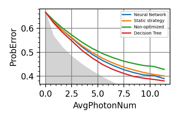
Fig. 39 alpha_bound=0.75, loss=1
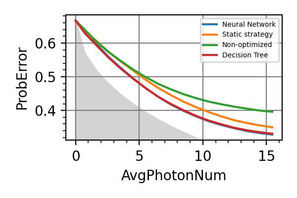
Fig. 40 alpha_bound=1.00, loss=1
The non-optimized strategy refers to a device where the phase imprinted by the beam-splitters are all zero and the reflectivity is chosen, so that the same fraction of the signal reaches each one of the photon counter.
There is an “adaptivity-gap” between the performances of the static controls and the two adaptive strategies (NN and decision tree). This gap starts from zero and grows with the average number of photons. This make sense, since with very few photons we don’t expect the adaptive measurements to be better than the static one, since almost always the measurement outcomes of the photon counters will be zero, which doesn’t give any information about the training states. On the other hand with many photons there is more space for learning. This can be also understood considering the number of possible trajectories of the particle filter ensemble during the estimation, which is one for
 ,
and grows with the number of photons.
More possible trajectories means
having different controls on each
one of them in order to improve the precision,
which is by definition adaptivity.
,
and grows with the number of photons.
More possible trajectories means
having different controls on each
one of them in order to improve the precision,
which is by definition adaptivity.In our experiments we observed that the convergence of the NN to the optimal strategy is slow and doesn’t always happen (see the case alpha_bound=0.75 in the figures), while the decision tree is shown to be a superior control for this device. In general, in a problem with many parameters and a relatively small space of possible outcome trajectories, the decision three is superior to the neural network. On the other hand with few parameters and a large space of outcome trajectories (like in the examples on NV centers) the decision three is unapplicable in the form we presented here and the NN is superior.
In the figure on the left the first nodes of the decision tree for alpha_bound=0.75 are shown. The controls from the decision tree have the advantage of being faster to compute with respect to those of the NN, but storing the tree requires more memory. A future work could be to trim the tree by keeping only the paths that correspond to the most probable trajectories (see the figure on the right).
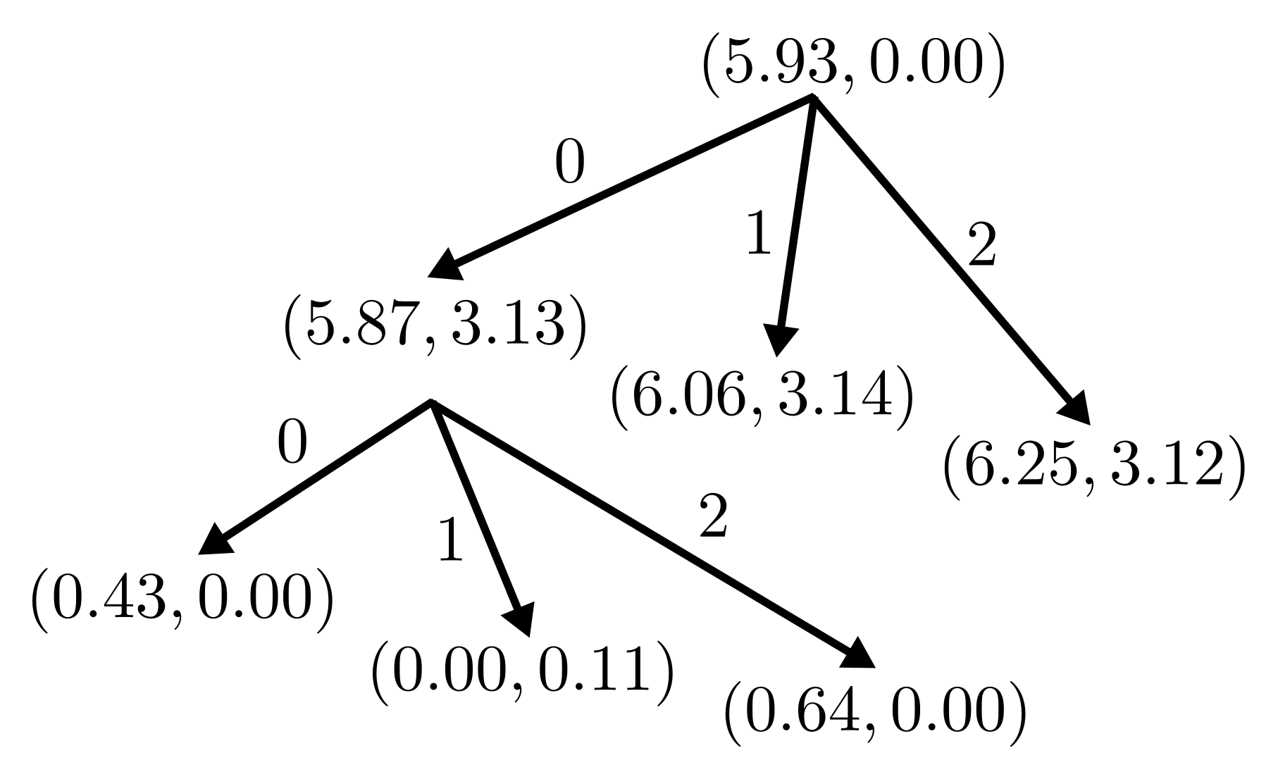
alpha_bound=0.75, decision tree
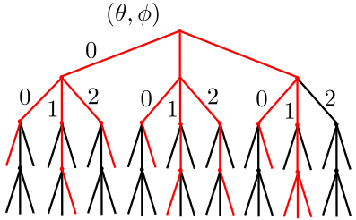
trimmed decision tree
In the following figure five trajectories for the neural network controls
and
are showed.
There is a tendency for the control trajectories
to diverge in time (this can be seen well in
the plot for ),
since having already done some
measurements means that the controls can be tailored
to the particular instance of the task.
This behaviour is trained in the
neural network but is hard coded
in the decision tree strategy.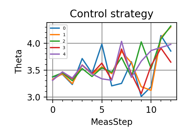
Fig. 41 alpha_bound=1.00, loss=1
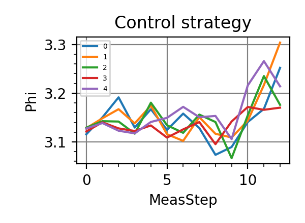
Fig. 42 alpha_bound=1.00, loss=1
The shaded grey areas in the above plot indicate the performances of the pretty good measurement, computed for multiple copies of the encoded states. This is not the ultimate precision bound regarding this discrimination problems, but it is a reasonable reference value not achievable with linear optics.
The fact the the training is able to find and exploit such small gain from the adaptivity speeks for the efficiency and power of the method.
Notes
For a large number of resources the error probability curves tend to saturate. This is because even with infinite num_ref and therefore perfect knowledge of the training states a single copy of the signal can’t be classified unambiguously.
For the estimation of seven parameter 512 particles in the ensamble are too few. Using 1024 particles improves the performances a bit, but not that much.
We mentioned that loss=1 always outperforms loss=0. This is because with loss=0 we assume that the error probability of the apparatus is the one estimated by the particle filter. In this way, however, the error probability is overeatimated.
In this example we are estimating multiple quantum incompatible parameters, that are the x and p components of the training states and the signal, whose corresponding generators don’t commute.
Known bugs: the training on the GPU freezes if the parameter alpha_bound is set to be too large. This is probably due to a bug in the implementation of the function random.poisson. A preliminary work-around has shown that reimplementing the extraction from a Poissonian distribution with random.categorical would solve the problem.
All the trainings of this module have been done on a GPU NVIDIA Tesla V100-SXM2-32GB or on a GPU NVIDIA GeForce RTX-4090-24GB, each requiring
hours.
- parse_args()
Arguments
- scratch_dir: str
Directory in which the intermediate models should be saved alongside the loss history.
- trained_models_dir: str = “./qml_classifier/trained_models”
Directory in which the finalized trained model should be saved.
- data_dir: str = “./qml_classifier/data”
Directory containing the csv files produced by the
performance_evaluation()and thestore_input_control()functions.- prec: str = “float64”
Floating point precision of the whole simulation.
- batchsize: int = 1024
Batchsize of the simulation.
- n: int = 64
Number of neurons per layer in the neural network.
- num_particles: int = 512
Number of particles in the ensemble representing the posterior.
- num_ref: int = 4
Number of copies of each training state
,
,
.- iterations: int = 32768
Number of training steps.
- simulation_qmlclassifier(args, alpha_bound: float = 1.0, learning_rate: float = 0.01, loss: int = 0, arch: str = 'serial')
Simulation of the QML classifier.
Parameters
- args:
Arguments passed to the Python script.
- alpha_bound: float = 1.0
Size of the hypercube of the admissible values for the real components of the three training states.
- learning_rate: float = 1e-2
Initial learning rate for the neural network. The static strategy has a fixed initial learning rate of 1e-1. Both are reduced during the training according to
InverseSqrtDecay.- loss: {0, 1}
Type of loss for the training. The two possibilities (loss=0, 1) are discussed in the documentation of the
loss_function()method.- arch: {“serial”, “parallel”}
Architecture of device. If it is “serial” then an object
QMLDiscriminatorSerialis instantiated for the simulation, if it is “parallel” instead, an objectQMLDiscriminatorParallelis instantiated.
Photonic circuit
- class FourModesCircuit(batchsize: int, params: List[Parameter], prec: str = 'float64', single_control: bool = False, num_photons: int = 1)
Bases:
StatelessPhysicalModel,PhotonicCircuitFour modes interferometer for the simultaneous estimation of three phases 8.
The interferometer has two balanced quarter as opening and closing elements, which are the generalization of the balanced beam splitter for four modes in input and four modes in output. The three unknown phases are called
 , while the
control phases are
, while the
control phases are  .
See also the picture in the documentation
of the
.
See also the picture in the documentation
of the PhotonicCircuitSimulationclass.Constructor of the
FourModesCircuitclass.Parameters
- batchsize: int
Number of simultaneous estimations of the phases.
- params: List[
Parameter] List of parameters to be estimated, passed to the class constructor. These must be the three unknown phases in the interferometer, with their respective priors.
- prec: str = {“float64”, “float32”}
Floating point precision of the simulation.
- single_control: bool = False
If this flag is active, then the three control phases in the interferometer, i.e.
, are all equal
to a single control phase  to
be optimized, i.e.
to
be optimized, i.e.
 .
.- num_photons: {1, 2, 3, 4}
Mean number of photons in the input state to the interferometer, which is always a collection of coherent states
 .
This parameter can take integer values
from 1 to 4 (extrema included), and the
corresponding input states are
.
This parameter can take integer values
from 1 to 4 (extrema included), and the
corresponding input states arenum_photons=1:
 ,
,
 ,
,num_photons=2:
 ,
,
 ,
,num_photons=3:
 ,
,
 ,
,num_photons=4:
 .
.
An average of one photon at most enters each line of the circuit.
Achtung!: The input states are not Fock states.
- count_resources(resources: Tensor, outcomes: Tensor, controls: Tensor, true_values: Tensor, meas_step: Tensor) Tensor
Each execution of the photonic circuit is counted as a consumed resource, and it is called a step.
- model(outcomes: Tensor, controls: Tensor, parameters: Tensor, meas_step: Tensor, num_systems: int = 1) Tensor
Returns the log-likelihood of getting a particular outcome for the photon counting measurements on each mode of the interferometer after the closing quarter.
Parameters
- outcomes: Tensor
Tensor of shape (bs, num_systems, 4) and type prec containing the number of photons to condition on for each of the four lines.
- controls: Tensor
If single_control=False this is a Tensor of shape (bs, num_systems, 3) and of type prec containing the three control phases, while if single_control=True this Tensor has shape (bs, num_systems, 1) and contains the single control phase.
- parameters: Tensor
Tensor of shape (bs, num_systems, 3) and type prec containing the ensemble particles for the three unknown phases.
- meas_step: Tensor
Tensor of shape (bs, num_systems, 1) and type prec. It is the index of the current execution of the interferometer and starts from zero. We call a single circuit execution, i.e. sending the input and measuring the outcome, a step.
- num_systems: int = 1
Number of circuits simulated for each batch element.
Returns
- prob: Tensor
Tensor of shape (bs, num_systems) and type prec containing the probability of getting outcomes as a results upon the execution of the photon counting measurement.
- perform_measurement(controls: Tensor, parameters: Tensor, meas_step: Tensor, rangen: Generator) Tuple[Tensor, Tensor]
The input state of the four bosonic modes is fed to the circuit and a photon counting measurement is performed on each output lines after the closing quarter.
Parameters
- controls: Tensor
If single_control=False this is a Tensor of shape (bs, 1, 3) and of type prec containing the three control phases, while if single_control=True this Tensor has shape (bs, 1, 1) and contains the single control phase.
- parameters: Tensor
Tensor of shape (bs, 1, 3) and type prec containing the true values of the three phases to be estimated
.- meas_step: Tensor
Tensor of shape (bs, 1, 1) and type prec. It is the index of the current execution of the interferometer and starts from zero. We call a single circuit execution, i.e. sending the input and measuring the outcome, a step.
- rangen: Generator
Random number generator from the module
tensorflow.random.
Returns
- outcomes: Tensor
Tensor of shape (bs, 1, 4) and type prec containing the number of photons observed in the photon counting measurement on each of the four lines.
- log_prob: Tensor
Tensor of shape (bs, 1) and type prec containing the logarithm of the probability of getting the observed number of photons.
- class PhotonicCircuit(batchsize: int, num_wires: int, prec: str = 'float64')
Bases:
CoherentStatesProgrammable multimode photonic circuit. Non-linear elements (other than photon counting) can’t be implemented. No homodyne measurement is available.
Constructor of the
PhotonicCircuitclass.Parameters
- batchsize: int
Number of simultaneous simulations of the circuit.
- num_wires: int
Number of bosonic lines in the circuit.
- prec: {“float64”, “float32”}
Floating point precision of the simulation.
- balanced_beamsplitter_line(state: Tensor, i: int, num_systems: int) Tensor
Applies a balanced beamsplitter without phase shift between two consecutive bosonic lines.
Parameters
- state: Tensor
Tensor of shape (bs, num_systems, 2 num_wires) of type prec containing the real components of the state of the num_wires bosonic modes. The x-components are the entries from 0 to num_wires-1, and the p-components the entries from num_wires to 2 num_wires-1.
- i: int
The balanced BS is applied between the i-th and the i+1-th line. The counting starts from zero.
- num_systems: int
Size of the second dimension of state. It is the number of circuits simulated for each element of the batch, i.e. for each estimation.
Returns
- state: Tensor
Tensor of shape (bs, num_systems, 2 num_wires) of type prec containing the evolved state of the photonic circuit after the application of the beamsplitter.
- beamsplitter_line(state: Tensor, theta: Tensor, phi: Tensor, i: int) Tensor
Controllable beamsplitter between two consecutive lines.
The symbol ? in the shape of a Tensor means that this dimension can have arbitrary size unknown to this method.
Parameters
- state: Tensor
Tensor of shape (bs, ?, 2 num_wires) of type prec containing the real components of the state of the num_wires bosonic modes. The x-components are the entries from 0 to num_wires-1, and the p-components the entries from num_wires to 2 num_wires-1.
- theta: Tensor
Tensor of shape (bs, ?) and of type prec. It contains the transmission coefficient of the BS. It is indicated with
.- phi:
Tensor of shape (bs, ?) and of type prec. It contains the phase applied by the BS. It is indicated with
.- i: int
The BS is applied between the i-th and the i+1-th line. The counting starts from zero.
Returns
- state: Tensor
Tensor of shape (bs, ?, 2 num_wires) of type prec containing the evolved state of the photonic circuit after the application of the beamsplitter.
- phase_shift_line(state: Tensor, phase: Tensor, i: int) Tensor
Controllable phase shift on the i-th bosonic mode.
The symbol ? in the shape of a Tensor means that this dimension can have arbitrary size unknown to this method.
Parameters
- state: Tensor
Tensor of shape (bs, ?, 2 num_wires) of type prec containing the real components of the state of the num_wires bosonic modes. The x-components are the entries from 0 to num_wires-1, and the p-components the entries from num_wires to 2 num_wires-1.
- phase: Tensor
Tensor of shape (bs, ?) and type prec containing the phase shift to be applied to the i-th bosonic mode.
- i: int
Index of the bosonic mode to be phase shifted. The counting starts from zero.
Returns
- state: Tensor
Tensor of shape (bs, ?, 2 num_wires) of type prec containing the evolved state of the photonic circuit.
- photon_counting_all(state: Tensor, rangen: Generator) Tuple[Tensor, Tensor]
Performs the photon counting on each line of the circuit individually.
Parameters
- state: Tensor
Tensor of shape (bs, 1, 2 num_wires) of type prec containing the real components of the state of the num_wires bosonic modes. The x-components are the entries from 0 to num_wires-1, and the p-components the entries from num_wires to 2 num_wires-1.
- rangen: Generator
Random number generator from the module
tensorflow.random.
Returns
- outcomes: Tensor
Number of photons observed on each line. It is a Tensor of shape (bs, 1, num_wires) and type prec.
- log_prob: Tensor
Log-likelihood of getting the observed outcomes upon the measurement. It is a Tensor of shape (bs, 1) and type prec.
- postselect_photon_counting_all(state: Tensor, outcomes: Tensor, num_systems: int = 1) Tensor
Postselection of the photon counting result on each line of the photonic circuit.
Parameters
- state: Tensor
Tensor of shape (bs, num_systems, 2 num_wires) of type prec containing the real components of the state of the num_wires bosonic modes. The x-components are the entries from 0 to num_wires-1, and the p-components the entries from num_wires to 2 num_wires-1.
- outcomes: Tensor
Tensor of shape (bs, num_systems, num_wires) and type prec containing the number of photons in each line to condition on.
- num_systems: int
Size of the second dimension of state. It is the number of circuits simulated for each element of the batch, i.e. for each estimation.
Returns
- log_prob: Tensor
Log-likelihood of getting outcomes as result upon the photon counting measurements. It is a Tensor of shape (bs, num_systems) and type prec.
- total_mean_phot(state: Tensor, num_systems: int) Tensor
Computes the total mean photon number in the photonic circuit.
Given a list of states
 for the bosonic line,
this method returns
for the bosonic line,
this method returns(80)

Parameters
- state: Tensor
Tensor of shape (bs, num_systems, 2 num_wires) of type prec containing the real components of the state of the num_wires bosonic modes. The x-components are the entries from 0 to num_wires-1, and the p-components the entries from num_wires to 2 num_wires-1.
- num_systems: int
Size of the second dimension of state. It is the number of circuits simulated for each element of the batch, i.e. for each estimation.
Returns
- Tensor:
Mean number of photons present in the entire circuit. It is a Tensor of shape (bs, num_systems) and type prec.
- class PhotonicCircuitSimulation(particle_filter: ParticleFilter, phys_model: FourModesCircuit, control_strategy: Callable, simpars: SimulationParameters, random: bool = False)
Bases:
StatelessMetrologySimulation for the
FourModesCircuitclass.Achtung! This
Simulationclass is implemented for unknown phases that are defined as discrete parameters, that is, that can take values only in a finite set. For this reason the task solved here is hypothesis testing.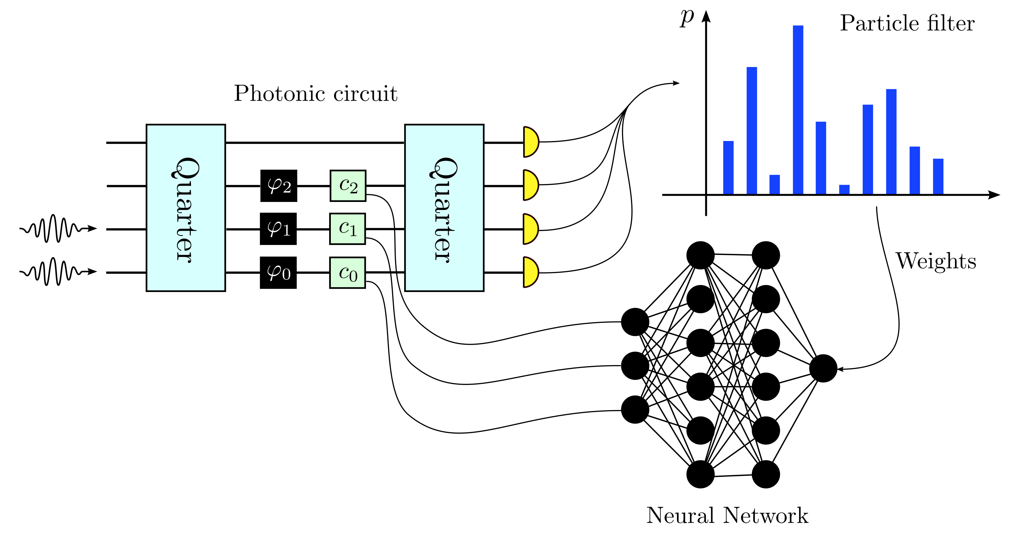
Given the number of possible values
 that each phase
can assume, i.e. the length of the
values attributes of their respective
that each phase
can assume, i.e. the length of the
values attributes of their respective
Parameterobjects, the total number of hypothesis to discriminate is . The particle
filter contains one and only one particle for
each hypothesis along with their
corresponding weights
. The particle
filter contains one and only one particle for
each hypothesis along with their
corresponding weights
 ,
that are updated with the Bayes rule
after each step.
,
that are updated with the Bayes rule
after each step.The posterior distribution on the hypothesis is the input to the control strategy. The loss function
loss_function()simply returns the probability of guessing the wrong hypothesis after all the measurements.Constructor of the
PhotonicCircuitSimulationclass.Parameters
- particle_filter:
ParticleFilter Particle filter responsible for the update of the Bayesian posterior on the hypothesis.
- phys_model:
FourModesCircuit Abstract description of the balanced four mode interferometer.
- control_strategy: Callable
Callable object (normally a function or a lambda function) that computes the values of the controls
for the next step.- simpars:
SimulationParameters Contains the flags and parameters that regulate the stopping condition of the measurement loop and modify the loss function used in the training.
- random: bool = False
If this flag is True a column of random numbers extracted uniformly in
![[0, 2 \pi]](_images/math/ba89b6876fcc1f99f2762f1fee49ed327e6bc912.svg) is appended to the
input_tensor generated by
is appended to the
input_tensor generated by
generate_input()for each control in the circuit. The number of controls can be either three or one according to the flag single_control of phys_model.
- generate_input(weights: Tensor, particles: Tensor, meas_step: Tensor, used_resources: Tensor, rangen: Generator) Tensor
Generates the input_tensor passed to control_strategy, on the basis which the next controls are predicted.
The input_tensor is composed on the following columns:
weights, i.e. the posterior distribution on the possible values of the phases. These are
 columns,
meas_step normalized in [-1, +1],
used_resources normalized in [-1, +1].
one or three columns of random numbers uniformly extracted in
 . This is present only
if random=True.
. This is present only
if random=True.
The shape of the returned input is (bs, input_size), with input_size being
 if random=False or
 if random=True and
single_control=False.
if random=True and
single_control=False.
- loss_function(weights: Tensor, particles: Tensor, true_values: Tensor, used_resources: Tensor, meas_step: Tensor) Tensor
Loss function for the hypothesis testing in the four arms interferometer.
On each estimation in the batch the loss is zero if the correct phases are guessed correctly and one if they are guessed wrongly. In symbols, given the delta function
(81)
the guess based on the Bayesian posterior is
(82)

and calling
the index of the
correct hypothesis for the phases values
the loss can be expressed as(83)

which, averaged on the batch is the error probability.
- particle_filter:
- main()
In the following we report the evaluated error probability in the correct identification of three phases in a four arms interferometer with various input states. Each phase can assume the two values
 .
The three phases
can be controlled,
see the picture in the documentation
of the
.
The three phases
can be controlled,
see the picture in the documentation
of the PhotonicCircuitSimulationclass, and the performances of three control strategies have been compared for the same input states.With this circuit we are testing in parallel for each slot whether a phase shift is there or not. This phase shift could be due to the presence of a certain object, a chemical species, or it could be a piece of codified information.
The following plots represent the probability of guessing the unknown phases wrong as a function of the mean number of photons consumed in the estimation and of the number of measurements, for the adaptive, the static, and the random strategies.
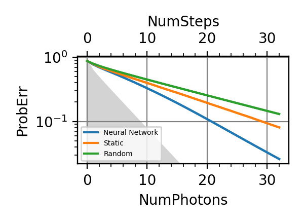
Fig. 43 num_photons=1
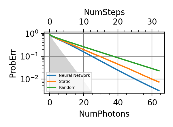
Fig. 44 num_photons=2
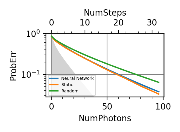
Fig. 45 num_photons=3
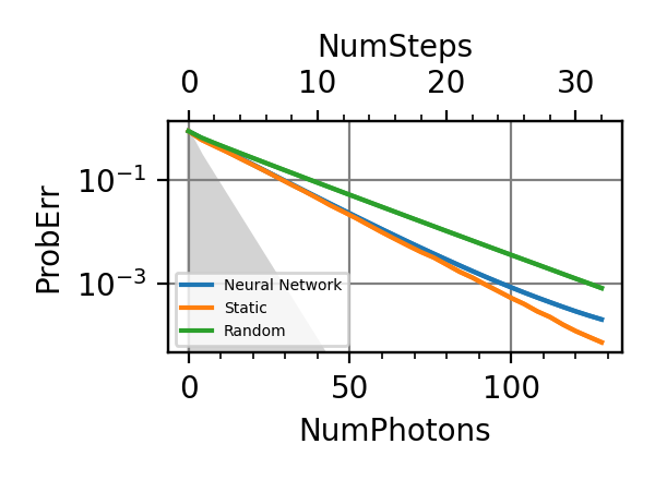
Fig. 46 num_photons=4
The shaded grey areas in the above plot indicate the performances of the pretty good measurement, computed for multiple copies of the encoded states. This is not the ultimate precision bound regarding this discrimination problems, but it is a reasonable reference value not achievable with linear optics.
Only for num_photons=1, 2 the adaptive strategy has been proven to give some advantage with respect to the static one. The state with three photons doesn’t perform well in comparison to all the other inputs. The best input in terms of the consumed number of photons to reach a certain probability error is the state with a single photon on average. It is possible that in terms of the damage caused to the sample or the energy used (which are both proportional to the total number of photons) performing many measures each with a vanishingly small photon number is optimal. This hypothesis should be verified with more simulations in the range num_photons<1. If it that is the case, then minimizing the energy or the damage would mean stretching the total measurement time, which could also be unfeasible beyond a certain amount. For a fixed number of measurements, therefore for a fixed estimation time, the states with many photons seem to perform better then those with less photons (num_photons=3 being an exception). The fact that for different resources either the states with many of with few photons are optimal underlines the importance of clearly identifying the resource when discussing metrology. Other simulations should be performed for the input states
 ,
,  and
and  to asses their
usefulness.
to asses their
usefulness.Notes
Known bugs: the training on the GPU freezes if the number of input photons is too large. This is probably due to a bug in the implementation of the function random.poisson. A preliminary work-around has shown that reimplementing the extraction from a Poissonian distribution with random.categorical would solve the problem.
All the training of this module have been done on a GPU NVIDIA Tesla V100-SXM2-32GB, each requiring
hours.
- parse_args()
Arguments
- scratch_dir: str
Directory in which the intermediate models should be saved alongside the loss history.
- trained_models_dir: str = “./photonic_circuit/trained_models”
Directory in which the finalized trained model should be saved.
- data_dir: str = “./photonic_circuit/data”
Directory containing the csv files produced by the
performance_evaluation()and thestore_input_control()functions.- prec: str = “float64”
Floating point precision of the whole simulation.
- batchsize: int = 4096
Batchsize of the simulation.
- n: int = 64
Number of neurons per layer in the neural network.
- num_steps: int = 32
Number of uses of the interferometer, i.e. number of measurements in the hypothesis testing.
- iterations: int = 32768
Number of training steps.
- photonic_circuit_estimation(args, learning_rate: float = 0.01, gradient_accumulation: int = 1, cumulative_loss: bool = True, phase_values: Tuple = (0, 1), single_control: bool = False, num_photons: int = 1)
Simultaneous estimation of three phases in the four arms interferometer as describe by the
FourModesCircuitclass.Each call to this function will perform the hypothesis testing on the values of the three phases for three strategies, i.e. the adaptive one implemented with a NN, the static, and the random strategies.
Parameters
- args:
Arguments passed to the Python script.
- learning_rate: float = 1e-2
Initial learning rate for the neural network. The static strategy has a fixed initial learning rate of 1e-1. Both are reduced during the training according to
InverseSqrtDecay.- gradient_accumulation: int = 1
Flag of the
train()function.- cumulative_loss: bool = True
Flag
cumulative_loss. Set for all the simulations.- phase_values: Tuple = (0, 1)
Contains the possible discrete values that each phase
 can assume
independently.
can assume
independently.- single_controls: bool = False
If the function is called with single_control=True, then it will evaluate the performances of the adaptive, random, and static strategies in the scenario where the three controllable phases are all equal, i.e.
,
and there is therefore only a single
scalar control . This flag is
used in the initialization of the
FourModesCircuitobject.- num_photons: int = 1
Mean number of photons in the input state of the interferometer for each measurement step. This values is used in the initialization of the
FourModesCircuitobject.
Linear Multiclassifier
- class ClassifierSimulation(particle_filter: ParticleFilter, phys_model: LinearMulticlassifier, control_strategy: Callable, simpars: SimulationParameters, random: bool = False)
Bases:
StatelessSimulationSimulation class associated to the
LinearMulticlassifierphysical model.Attributes
- bs: int
Batchsize of the simulation.
- phys_model:
LinearMulticlassifier Parameter phys_model passed to the class constructor.
- control_strategy: Callable
Parameter control_strategy passed to the class constructor.
- pf:
ParticleFilter Parameter particle_filter passed to the class constructor.
- input_size: int
This attribute depends on the flag random. If random=False then input_size=1 while if random=True then input_size=2 phys_model.num_wires^2.
- input_name: List[str]
If random=False then this list contains only the string “MeasStepOverMaxStep”, while if random=True then it contains the name of all the BS network parameters, i.e.
 and
and  for
for
 and
and

- simpars:
SimulationParameters Parameter simpars passed to the class constructor.
- num_layers: int
Number of BS layers in the signal estimation. It is the
num_stepsattribute of simpars. It is indicated also with in the formulas.- random: bool = False
Flag random passed to the class constructor.
Constructor of the
ClassifierSimulationclass.Parameters
- particle_filter:
ParticleFilter Particle filter responsible for the update of the Bayesian posterior on the hypothesis.
- phys_model:
LinearMulticlassifier Abstract description of the linear multiclassifier.
- control_strategy: Callable
Callable object (normally a function or a lambda function) that computes the values of the controls for the next measurement from the Tensor input_strategy. If random=False then input_strategy contains only the (renormalized) index of the current layer and the control_strategy should return the corresponding BS parameters to be optimized. If on the other hand random=True input_strategy contains a randomly extracted parametrization of a BS network, that control_strategy can immediately return.
- simpars:
SimulationParameters Contains the flags and parameters that regulate the stopping condition of the measurement loop and modify the loss function used in the training.
- random: bool = False
If this flag is True the 2 phys_model.num_wires^2 randomized controls for the BS network are added to the output of the
generate_input()method.
- generate_input(weights: Tensor, particles: Tensor, meas_step: Tensor, used_resources: Tensor, rangen) Tensor
Builds the input_strategy tensor.
If random=False this method returns
 , where
is meas_step, i.e. the index of the current layer
and is the total number of layers, i.e.
the attribute num_layers.
This is a Tensor of shape (bs, 1) and type prec
, where
is meas_step, i.e. the index of the current layer
and is the total number of layers, i.e.
the attribute num_layers.
This is a Tensor of shape (bs, 1) and type precIf, on the other hand, random=True this method returns
 randomly extracted angles
in
randomly extracted angles
in  , which identify a BS network.
This is a Tensor of shape
(bs, 2 phys_model.num_wires^2)
and type prec.
, which identify a BS network.
This is a Tensor of shape
(bs, 2 phys_model.num_wires^2)
and type prec.
- loss_function(weights: Tensor, particles: Tensor, true_values: Tensor, used_resources: Tensor, meas_step: Tensor) Tensor
After all the measurements have been performed the particle filter contains a discrete distribution of posterior probabilities for the signal classes, i.e.
 .
The guess for the signal class is defined by the
function
.
The guess for the signal class is defined by the
function(84)

and the loss is
(85)

with
(86)
Averaged on many batch
 approximates the error probability.
- class LinearMulticlassifier(batchsize: int, list_alphas: Tuple[complex], prec: str = 'float64')
Bases:
StatelessPhysicalModel,PhotonicCircuitModel for a network of beam splitters (BS) and phase shifts that receives as input the signal
to be classified, with
 being the classes. The number
  is the attribute
num_hypothesis and the length
of the tuple list_alphas passed to the
constructor.
is the attribute
num_hypothesis and the length
of the tuple list_alphas passed to the
constructor.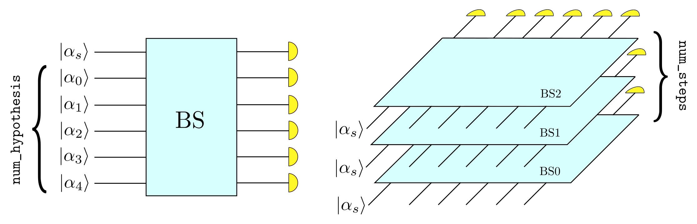
The other inputs of the network are in order
,
, ,
…,  , that is,
the reference states corresponding to the
possible hypothesis (classes), which,
at difference with the example of the
, that is,
the reference states corresponding to the
possible hypothesis (classes), which,
at difference with the example of the
dolinar_threeare fixed for each execution of the task. It follows that the network has wires. The output of
the network is measured with
individual photon counters on each wire.
wires. The output of
the network is measured with
individual photon counters on each wire.The signal
will
be classified according to the photon counters
outcomes. If more than one signal state
is available multiple BS networks can be stacked
on one another and the classification will be based
on the measurements on all the layers.
Each layer can have a different network
BS0, BS1, …Attributes
- bs: int
Batchsize of the simulation.
- list_alphas: Tuple[complex]
List of reference states. It is a parameter passed to the class constructor.
- num_hypothesis: int
Number of classes or hypothesis. It is the length of the tuple list_alphas. It is also indicated with the symbol
.- num_wires: int
Number of wires in the network. It is num_hypothesis+1, i.e.
.- controls: List[
Control] Real parameters identifying the BS network.
- params: List[
Parameter] Contains the description of the unknown to be estimated, i.e. the discrete parameter Signal that takes values in the set
 .
The initial value randomization must be
disabled in this application,
i.e. the flag randomize of the
.
The initial value randomization must be
disabled in this application,
i.e. the flag randomize of the
Parameterconstructor must be set to False. In this way initializing particle in the ParticleFilterwill produce particles with values in this order and
without repetitions.
in this order and
without repetitions.- controls_size: int
Number of real parameters of the BS network, i.e.
.- d: int = 1
Number of unknown parameters to estimate, i.e. one, the signals class.
- outcomes_size: int
Number of scalar outcomes for each layer of networks, i.e. the number of wires
.- prec: str
Floating point precision of the controls, outcomes, and parameters.
Constructor of the
LinearMulticlassifierclass.Parameters
- batchsize: int
Number of simultaneous estimations.
- list_alphas: Tuple[complex]
Tuple of complex numbers
 that represent the reference states.
- prec: = {“float64”, “float32”}
Floating point precision of the controls, outcomes, and parameters.
- count_resources(resources: Tensor, outcomes: Tensor, controls: Tensor, true_values: Tensor, meas_step: Tensor) Tensor
The execution of each BS layer is counted as a consumed resource.
- model(outcomes: Tensor, controls: Tensor, parameters: Tensor, meas_step: Tensor, num_systems: int = 1) Tensor
Returns the probability of getting a certain number of photons after the application of the BS network to the input state
 .
.Parameters
- outcomes: Tensor
Tensor of shape (bs, num_systems, num_wires) and type prec containing the number of photons measured on each wire of the system after the application of the network.
- controls: Tensor
Tensor of shape (bs, num_systems, 2 num_wires^2) and type prec that parametrizes the BS network.
- parameters: Tensor
Tensor of shape (bs, num_systems, 1) and type prec that contains the class s of the signal
for each particle in
the particle filter ensemble.- meas_step: Tensor
Tensor of shape (bs, num_systems, 1) and type int32 that contains the index of the current BS layer. It starts from zero.
- num_systems: int = 1
Number of BS networks processed per batch.
Returns
- prob: Tensor
Tensor of shape (bs, num_systems) of type prec containing the probabilities of getting the number of photons outcomes after the BS network defined by controls has been applied on the signal defined by parameters.
- perform_measurement(controls: Tensor, parameters: Tensor, meas_step: Tensor, rangen: Generator) Tuple[Tensor, Tensor]
Application of the BS network to the input state
 and subsequent photon counting
measurements on all the wires.
and subsequent photon counting
measurements on all the wires.Parameters
- controls: Tensor
Tensor of shape (bs, 1, 2 num_wires^2) and type prec that parametrizes the BS network.
- parameters: Tensor
Tensor of shape (bs, 1, 1) and type prec that contains the class s of the signal
for each element of
the batch.- meas_step: Tensor
Tensor of shape (bs, 1, 1) and type int32 that contains the index of the current BS layer. It starts from zero.
- rangen: Generator
Random number generator from the module
tensorflow.random.
Returns
- outcomes: Tensor
Tensor of shape (bs, 1, num_wires) and type prec containing the number of photons measured on each wire of the system after the application of the BS network.
- log_prob: Tensor
Tensor of shape (bs, 1) and type prec containing the logarithm of the probability of getting the observed number of photons (the likelihood).
- bs_network_classify(args, batchsize: int, list_alphas: Tuple[complex], learning_rate: float = 0.1)
Runs the training of the linear multiclassifier for the list of reference states list_alphas. Compares the performances of the trained BS networks with that of randomly extracted networks.
Parameters
- args:
Arguments passed to the Python script.
- batchsize: int
Number of simultaneous classifications.
- list_alphas: Tuple[complex]
Tuple of complex numbers
that represent the reference states.- learning_rate: float = 1e-1
Initial learning rate for the training of the BS network. The learning rate is reduced during the training according to
InverseSqrtDecay.
Notes
Known bugs: the training on the GPU freezes if the number of photons in the apparatus is too large. This is probably due to a bug in the implementation of the function random.poisson. A preliminary work-around has shown that reimplementing the extraction from a Poissonian distribution with random.categorical would solve the problem.
At difference with other examples we haven’t used a neural network here, and therefore we don’t have adaptivity.
All the training of this module have been done on a GPU NVIDIA Tesla V100-SXM2-32GB, each requiring
hours.
- main()
The linear multiclassifier has been trained and tested for some symmetric configurations of the
 . In particular the roots
of the unit for
. In particular the roots
of the unit for  have
been chosen. For a symmetric configuration of
states the pretty good measurement (PGM) is optimal,
but it can’t be achieved with linear optics.
The optimality of the PGM means that a single layer
BS network can’t achieve the performances of the
PGM, however this raises the interesting question
of how many layers
(and copies of the signal )
are necessary to match or surpass the
error probability of the PGM.
Beside that, the performances of the trained BS
networks are also compared to that of randomly
extracted networks.
have
been chosen. For a symmetric configuration of
states the pretty good measurement (PGM) is optimal,
but it can’t be achieved with linear optics.
The optimality of the PGM means that a single layer
BS network can’t achieve the performances of the
PGM, however this raises the interesting question
of how many layers
(and copies of the signal )
are necessary to match or surpass the
error probability of the PGM.
Beside that, the performances of the trained BS
networks are also compared to that of randomly
extracted networks.The following plots represent the error probability in the classification of the signal versus the number of layers of the linear multiclassifier (a single “resources” is the execution of a layer).
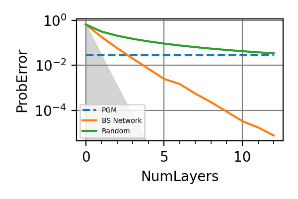
Fig. 47 m=3
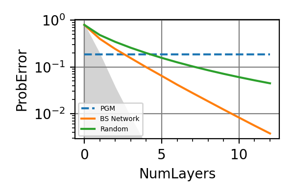
Fig. 48 m=5
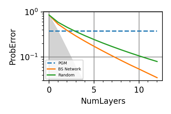
Fig. 49 m=7
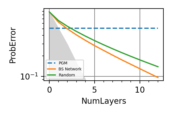
Fig. 50 m=9
The shaded grey areas in the above plot indicate the error probability of the PGM for many copies of the signal.
Three copies of the signal are always sufficient in these examples to match the PGM error probability. An interesting observation is that the advantage over the random strategy that the trained network has, decreases as the number of hypothesis grows. For
 we expect to have no gain. An adaptive strategy
may be able to restore the gap with the untrained
BS networks.
we expect to have no gain. An adaptive strategy
may be able to restore the gap with the untrained
BS networks.This example has been suggested to us by L. Bagnasacco.
Notes
In this example we are estimating two quantum incompatible parameters, that are the x and p components of the signal state, whose corresponding generators don’t commute.
All the training of this module have been done on a GPU NVIDIA Tesla V100-SXM2-32GB, each requiring
hours.
- parse_args()
Arguments
- scratch_dir: str
Directory in which the intermediate models should be saved alongside the loss history.
- trained_models_dir: str = “./linear_multiclassifier/trained_models”
Directory in which the finalized trained model should be saved.
- data_dir: str = “./linear_multiclassifier/data”
Directory containing the csv files produced by the
performance_evaluation()and thestore_input_control()functions.- prec: str = “float64”
Floating point precision of the whole simulation.
- batchsize: int = 8192
Batchsize of the simulation.
- num_layers: int = 12
Maximum number of layers of BS network.
- iterations: int = 4096
Number of training steps.
Optical Cavity
- class CavityParameters(delta_time: float, kappa: float, chi: float, num_photons: float, init_displacement: float, omega: float)
Bases:
objectPhysical parameters of the optical cavity.
- chi: float
Squeezing parameter of the non-linear crystal inside the cavity.
- delta_time: float
Time between two consecutive homodyne detections.
- init_displacement: float
Magnitude of the initial displacement of the cavity state in the phase space along the direction (1, 1).
- kappa: float
Fraction of the signal extracted at each homodyne measurement per second.
- num_photons: float
Thermal noise in the initial state of the cavity, i.e. number of photons in the thermal state.
- omega: float
Detuning between the cavity and the driving laser frequencies. It is the parameter to be sensed.
- class OpticalCavity(batchsize: int, params: List[Parameter], cav_parameters: CavityParameters, prec: str = 'float64')
Bases:
StatefulPhysicalModelAbstract model for an optical cavity with a single mode, that can be measured via homodyne detection.
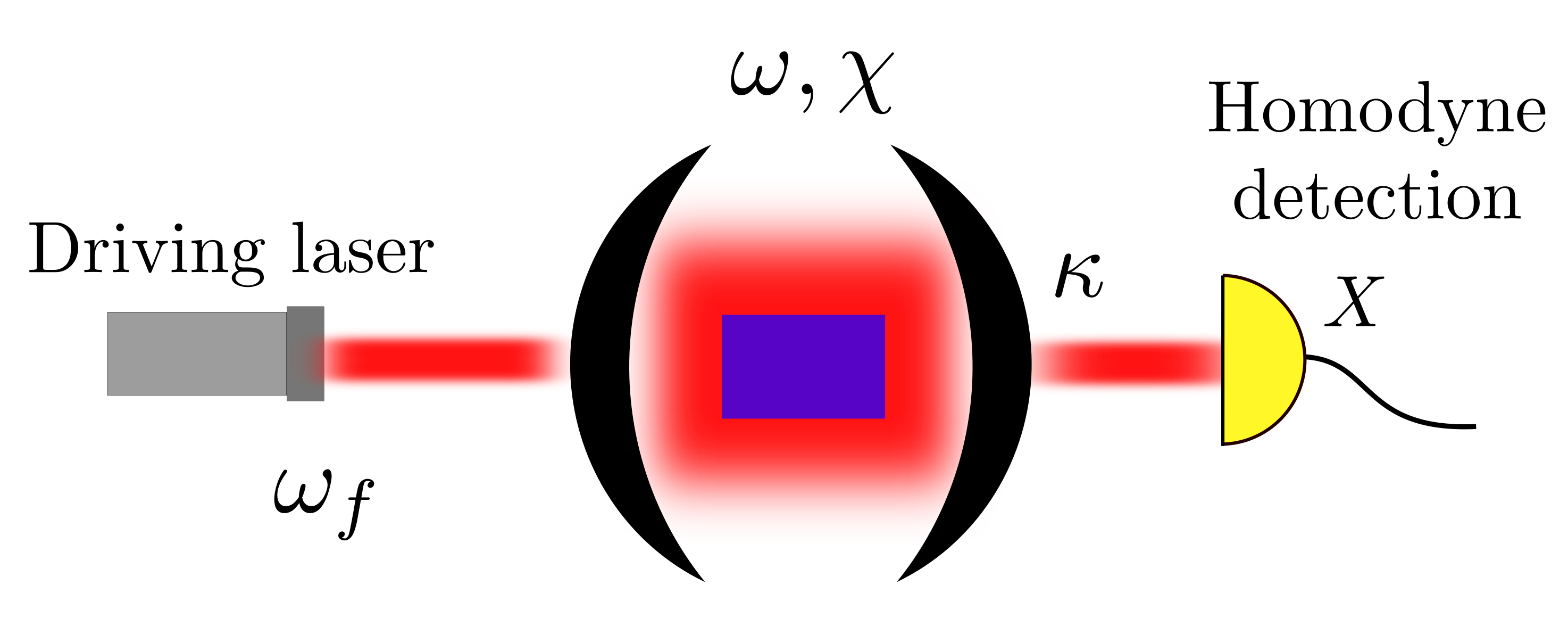
This model is taken from the paper of Fallani et al. 9.
- 9
A. Fallani, M. A. C. Rossi, D. Tamascelli, and M. G. Genoni, PRX Quantum 3, 020310 (2022).
Constructor of the
OpticalCavityclass.Parameters
- batchsize: int
Number of simultaneous estimations of the detuning frequency.
- params: List[
Parameter] List of unknown parameters to be estimated in the optical cavity experiment. It should contain the parameter Omega, i.e. the detuning frequency, with a single possible admissible value, that is the point at which the sensing is performed.
- cav_parameters:
CavityParameters Contains the values of the physical parameters of the cavity.
- prec: {“float64”, “float32”}
Floating point precision of the estimation.
- count_resources(resources: Tensor, outcomes: Tensor, controls: Tensor, true_values: Tensor, state: Tensor, meas_step: Tensor) Tensor
The consumed resource is the total evolution time. We consider the measurements instantaneous and spaced of
 . Therefore
measurements consume a total
amount of time
. Therefore
measurements consume a total
amount of time  .
.
- initialize_state(parameters: Tensor, num_systems: int) Tensor
Initialization of the cavity state.
The initial state of the cavity is Gaussian and so are all the operations performed on it, therefore it remains Gaussian. Accordingly the state can be described with the covariance matrix
 and the
displacement vector
and the
displacement vector  .
This method returns the initial state
of the cavity described by
.
This method returns the initial state
of the cavity described by(87)

where
 is
is
init_displacementand is
is
num_photons.Parameters
- parameters: Tensor
Tensor of shape (bs, num_systems, 1) containing the values of Omega. It is not used for producing the initial state.
- num_systems: int
Size of the second dimension of parameters. It is the number of cavity states instantiated for each batch element, i.e. for each estimation.
Returns
- initial_state:
Tensor of shape (bs, num_systems, 6) containing tha flattened and concatenated displacement vector
 and
covariance matrix
of cavity initial Gaussian state.
and
covariance matrix
of cavity initial Gaussian state.
- model(outcomes: Tensor, controls: Tensor, parameters: Tensor, state: Tensor, meas_step: Tensor, num_systems: int = 1) Tuple[Tensor, Tensor]
Returns the probability for the homodyne detection on the cavity field to give a certain outcome.
Parameters
- outcomes: Tensor
Tensor of shape (bs, num_systems, 1) and type prec containing the outcomes of the homodyne measurement to postselect on.
- controls: Tensor
Tensor of shape (bs, num_systems, 1) and type prec containing the feedback frequency
 of the
driving laser.
of the
driving laser.- parameters: Tensor
Tensor of shape (bs, num_systems, 1) and type prec containing the detuning frequency
of the
cavity at which the point
estimation is performed.- state: Tensor
Tensor of shape (bs, num_systems, 6) and type prec containing the displacement vector and the covariance matrix of the Gaussian state of the cavity.
- meas_step: Tensor
Tensor of shape (bs, num_systems, 1) and type prec. It is the index of the current homodyne measurement and it starts from zero.
- num_systems: int = 1
Number of optical cavities simulated per batch, i.e per estimation.
Returns
- prob:
Probability for the homodyne detection to return outcomes after the state has been evolved for a time
. It is a Tensor
of shape (bs, num_systems) and
type prec.- state:
State of the cavity conditioned on the observation of outcomes. It is a Tensor of shape (bs, num_systems, 6) and of type prec.
- perform_measurement(controls: Tensor, parameters: Tensor, true_state: Tensor, meas_step: Tensor, rangen: Generator) Tuple[Tensor, Tensor, Tensor]
Evolves the cavity for a time
, then
performs a homodyne detection
on the fraction of the cavity field
that leaks out through the partially
reflective mirror.For each measurement the state of the cavity is virtually splitted on a beam-splitter with transmission coefficient
 ,
where is
,
where is
delta_timeand is
is
kappa. The reflected part stays in the cavity, while the transmitted part is measured through homodyne detection, which causes a backreaction on the light remaining in the cavity (because of the squeezing of the cavity mode).Parameters
- controls: Tensor
Tensor of shape (bs, 1, 1) and type prec containing the feedback frequency
of the driving laser.- parameters: Tensor
Tensor of shape (bs, 1, 1) and type prec containing the detuning frequency
of the cavity,
at which the point
estimation must be performed.- true_state: Tensor
Tensor of shape (bs, 1, 6) and type prec containing the displacement vector and the covariance matrix of the Gaussian state of the cavity at the moment of the call of this method.
- meas_step: Tensor
Tensor of shape (bs, 1, 1) and type prec. It is the index of the current homodyne measurement and it starts from zero.
- rangen: Generator
Random number generator from the module
tensorflow.random.
Returns
- u: Tensor
Tensor of shape (bs, 1, 1) and type prec that contains the outcome of the homodyne detection on the cavity mode.
- log_prob: Tensor
Log-likelihood of having observed the outcome u. It is a Tensor of shape (bs, 1) and type prec.
- true_state: Tensor
Evolved state of the cavity after the application of the backreaction. It is a Tensor of shape (bs, 1, 6) and type prec.
- unitary_evolution(state: Tensor, parameters, controls, num_systems: int = 1) Tensor
Returns the state of the cavity after the unitary evolution of time duration
delta_time, with external driving.The evolution of the Gaussian state of the cavity due to the detuning and the non-linear crystal is described by the following differential equations for
 and
and  :
:(88)

(89)

with
(90)

where
 is
is
chi, i.e. the squeezing parameter, and is
omega, i.e. the detuning. is the parameter controls
and is determined by the external driving.These differential equations can be solved exactly:
(91)

(92)

where
is
delta_time, i.e. the evolution time.Parameters
- state: Tensor
Tensor of shape (bs, num_systems, 6) containing the evolved state of the cavity before the evolution. It is the concatenation of the flattened versions of the moments
and the covariance matrix
 .
.- parameters: Tensor
Tensor of shape (bs, 1, 1) containing the value of the detuning frequency
.- num_systems: int = 1
Number of optical cavities simulated per batch element, i.e. per estimation.
Returns
- state: Tensor
Tensor of shape (bs, num_systems, 6) containing the evolved state of the cavity. It is the Tensor obtained by concatenating the flattened versions of
 and
and  .
.
Notes
In order to compute the exponential of the traceless matrix
 there is an handy
formula:
there is an handy
formula:(93)

where
 is the determinant
of
is the determinant
of  . This formula works for both
 and
and  .
.
- main()
We trained both the adaptive and the static strategies for controlling the feedback frequency and we found no advantage in using a neural network for all the values of
that we have explored.
In the following we report on the left
the Fisher information
per unit of time, i.e.
 as a function of the
evolution time
for the optimal adaptive strategies,
and on the right a plot
of the squeezing parameter
as a function of the
evolution time
for the optimal adaptive strategies,
and on the right a plot
of the squeezing parameter(94)

computed as function of time.
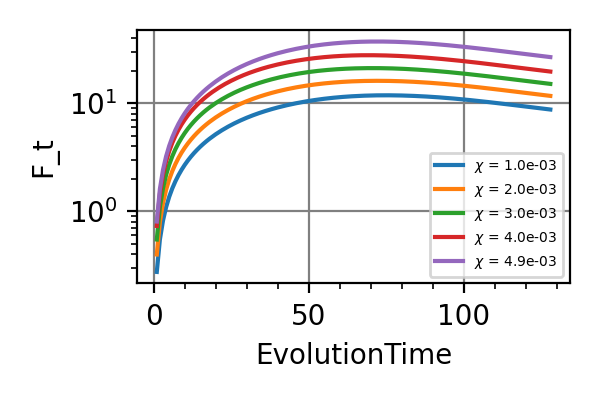
Fig. 51 Fisher/Time
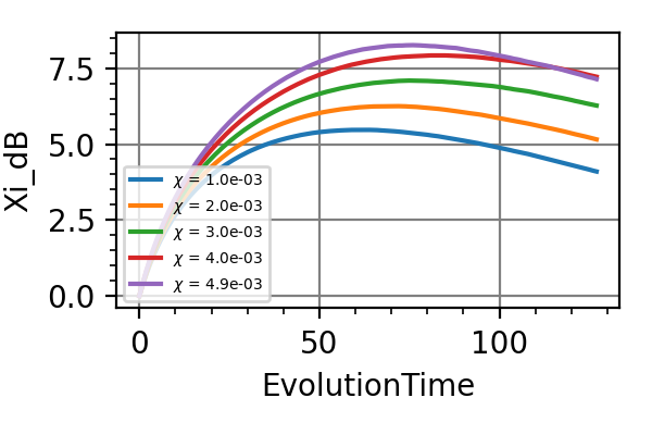
Fig. 52 Squeezing parameter
The point of the optimal strategies is to create squeezing on the x-axis (the one measured by the homodyne detection) and position the state on the p axis as far as possible from the origin, so that the rotation sensitivity is maximized.
In the following plots we report the mean value of the displacement in the phase space for the cavity state, always as a function of time.
At the very beginning the states spread on the x-axis due to the relative high initial thermal noise and the homodyne measurement backreaction, but at the end the controls have managed to give the states a p-components and to reduce the displacement along the x-axis.
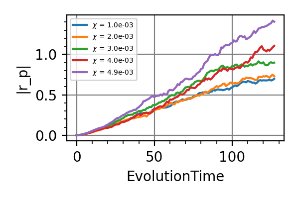
Fig. 53 Mean of
 .
.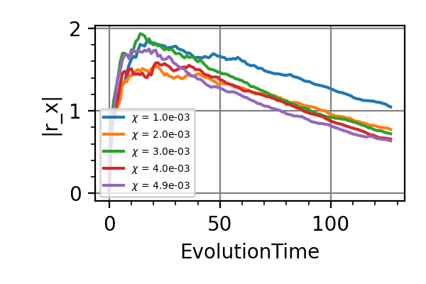
Fig. 54 Mean of
 .
.Notes
If instead of fixing
we had a interval of possible values for the parameter,
i.e. by setting the flag interval of the
function optimize_optical_cavity(), the neural network would be useful to modulate the optimal strategy as a function of.All the training of this module have been done on a GPU NVIDIA Tesla V100-SXM2-32GB, each requiring
hours.
- optimize_optical_cavity(args, chi: float, interval: bool = False)
Training of the optimal controls for the feedback frequency of the driving laser in the cavity in order to minimize the Cramér-Rao (CR) bound. This function evaluates the performances of a trained neural network, of a static (open-loop) strategy, and of the random controls.
While the squeezing parameters
is variable and passed to the call of
the function through the
parameter chi, all the other attributes
of CavityParametersare fixed to .
.With approximately 1% of the cavity field measured by the homodyne detection at every step we are in the regime of continuous measurements.
Parameters
- args:
Arguments passed to the Python script.
- chi: float
Squeezing parameter of the non-linear crystal in the cavity.
- interval: bool = False
If this flag is True, the minimization of the CR bound is done in the range of detuning frequency
 .
.
- parse_args()
Arguments
- scratch_dir: str
Directory in which the intermediate models should be saved alongside the loss history.
- trained_models_dir: str = “./optical_cavity/trained_models”
Directory in which the finalized trained model should be saved.
- data_dir: str = “./optical_cavity/data”
Directory containing the csv files produced by the
performance_evaluation()and thestore_input_control()functions.- prec: str = “float64”
Floating point precision of the whole simulation.
- n: int = 64
Number of neurons per layer in the neural network.
- batchsize: int = 16
Batchsize of the simulation.
- evolution_time: int = 128
Total evolution time of the cavity.
- learning_rate: float = 1e-2
Initial learning rate for the neural network.
- iterations: int = 1024
Number of training steps.
CFSK Receiver
- class CFSKReceiver(batchsize: int, alphabet_length: int, total_time_pulse: float, average_photon_number: float, delta_t: float, transmittance: float, delta_omega: float, delta_phase: float, time_extention_coefficient: int = 10, control_nullifier_tolerance: float = 0.0001, prec: str = 'float64')
Bases:
StatefulPhysicalModelModel for the M-ary coherent frequency shift keying (CFSK) detector. The system is stateful as the probability of observing a photon in a certain time-bin depends on the time of the last observation.
Constructor of the
CFSKReceiverclass.Parameters
- batchsizeint
Number of receivers simulated at the same time in the batch.
- alphabet_lengthint
Number of messages to be discriminated.
- total_time_pulsefloat
Duration of the pulse.
- average_photon_numberfloat
Average number of photons of the signal.
- delta_tfloat
Approximate time resolution of the detector. Because of how the computation of the probability is implemented, the actual time resolution will be slightly lower than this value, i.e. slightly better.
- transmittancefloat
Transmittance of the unbalanced beam splitter.
- delta_omegafloat
Frequency shift for each hypothesis.
- delta_phasefloat
Phase shift for each hypothesis.
- time_extention_coefficientint, optional
The probability density for observing a photon at a certain time is truncated to zero after a time interval
time_cut = total_time_pulse * time_extention_coefficient, starting from the time of detection of the last photon. This density is normalized to one in[time_last_photon, time_cut], so that a photon is always observed within the timetime_cut, even if the total number of photons in the signal is vanishingly small.This behavior is unphysical, but it is introduced to sample effectively from the said distribution. In the model, this behavior is corrected “by hand”, so that the probability of observing a photon within the time
total_time_pulseis exactly zero for a vanishing photon number.- control_nullifier_tolerancefloat, optional
If the effective controls of the modulated coherent state are less than this threshold, the probability of observing a photon for the rest of the pulse is set to zero exactly.
- precstr, optional
Floating-point precision of the model.
- count_resources(resources: Tensor, outcomes: Tensor, controls: Tensor, true_values: Tensor, state: Tensor, meas_step: Tensor) Tensor
The resource is the elapsed time since the beginning of the pulse.
Through the variable state, we determine whether a photon was measured outside the time duration of the pulse. In such cases, the resource is set to its maximum value total_time_pulse, and this constitutes the final measurement. The Bayesian posterior is updated with the information that no photon was observed within the duration of the pulse.
For the remaining simulations that have not yet reached the final step, the consumed amount of resource is zero. Only two resource values are possible: zero, which is not processed by performance_evaluation, and the maximum possible resource value, total_time_pulse, to which the final error probability is associated.
- initialize_state(parameters: Tensor, num_systems: int) Tensor
State initialization for the receiver. It contains just a single float, which is the time of last detection of a photon. It is initialized to zero.
Notes
The state of the receiver is an observed quantity, in contrast to quantum mechanical states, which are not observed.
- model(outcomes: Tensor, controls: Tensor, parameters: Tensor, state: Tensor, meas_step: Tensor, num_systems: int = 1)
Probability of observing the photon in the time bin indexed by outcome in the CFSK experiment.
Parameters
- outcomes: Tensor
Index of the time bin in which the last photon has been observed. Shape (bs, num_systems, 1) and type prec.
- controls: Tensor
Frequency and phase control for the current photon detection. Shape (bs, num_systems, 1) and type prec.
- parameters: Tensor
Messagges to be decoded. Shape (bs, num_systems, 1) and type prec.
- state: Tensor
Time of the last photon detection. Shape (bs, num_systems, 1) and type prec.
- meas_step: Tensor
Number of collected photons up to the point of calling the function minus one. Shape (bs, num_systems, 1) and type prec.
- num_systems: int = 1
Number of estimations simulated per batch.
Returns
- prob: Tensor
Probabilities associated to the observed time of detection of the photons. Tensor of shape (bs, num_systems) and type prec.
- state: Tensor
Detection time of the last photon. Tensor of shape (bs, num_systems, 1) and type prec.
- perform_measurement(controls: Tensor, parameters: Tensor, true_states: Tensor, meas_step: Tensor, rangen: Generator)
Stochastically extracts the time of detection of the next photon.
Parameters
- controls: Tensor
Controls for the frequency and phase of the coherent state to be added to the signal. Shape (bs, 1, 2) and type prec.
- parameters: Tensor
Message to be deciphered. Shape (bs, 1, 1) and type prec.
- true_states: Tensor
Time of detection of the last photon. Shape (bs, 1, 1) and type prec.
- meas_step: Tensor
Number of collected photons up to the point of calling the function minus one. Shape (bs, 1, 1) and type prec.
- rangen: Generator
Random number generator.
Returns
- outcomes: Tensor
Tensor of integers (casted to prec type) that contains the position of the extracted value in range_times. This is an internal index used to represent the time bin in which the detection occourred. Shape (bs, 1, 1) and type prec.
- log_prob: Tensor
Logarithm of the probability of the observed time for the photon detection. Shape (bs, 1) and type prec.
- true_state: Tensor
Detection time of the current photon. Shape (bs, 1, 1) and type prec.
- class CFSKSimulation(particle_filter: ParticleFilter, phys_model: CFSKReceiver, control_strategy: Callable, simpars: SimulationParameters)
Bases:
StatefulSimulationSimulation class for the CFSK receiver. It works with a
ParticleFilterand aCFSKReceiverobjects.Constructor of the
CFSKSimulationclass.Parameters
- particle_filter:
ParticleFilter Particle filter responsible for the update of the Bayesian posterior on the message.
- phys_model:
CFSKReceiver Model of the CFSK receiver.
- control_strategy: Callable
Control for the frequency and phase of the local oscillator.
- simpars:
SimulationParameters Parameter simpars passed to the class constructor.
- generate_input(weights: Tensor, particles: Tensor, state_ensemble: Tensor, meas_step: Tensor, used_resources: Tensor, rangen: Generator)
The input is the full posterior probability distribution on the set of discrete hypothesis.
- loss_function(weights: Tensor, particles: Tensor, true_state: Tensor, state_ensemble: Tensor, true_values: Tensor, used_resources: Tensor, meas_step: Tensor)
The loss function is the categorical classification error for the recovery of the message.
- particle_filter:
- cfsk_simulation(args, alphabet_length: int = 16, total_time_pulse: float = 1.0, average_photon_number: float = 4.0, delta_t: float = 0.01, learning_rate: float = 0.01)
Simulation of the receiver.
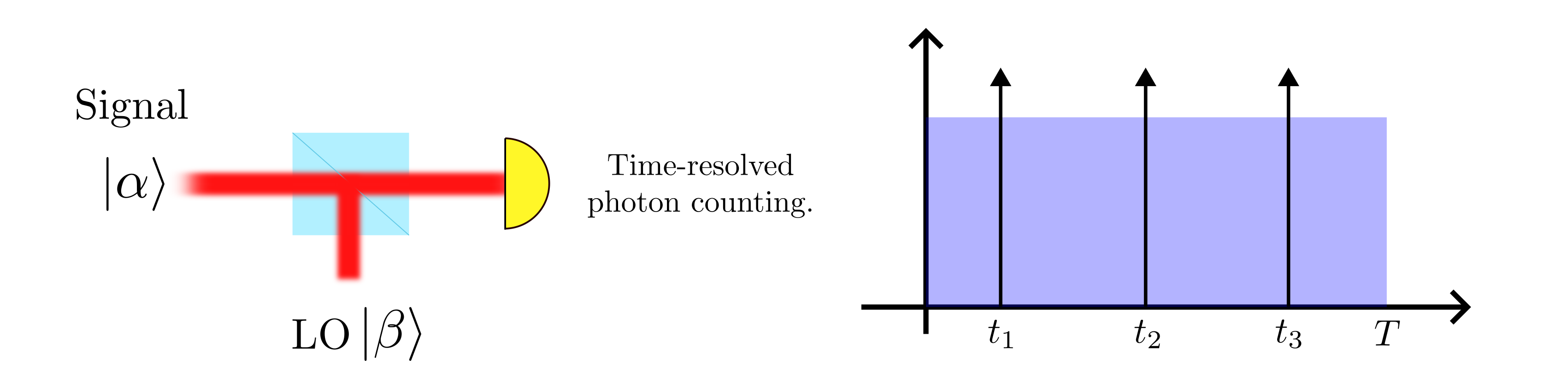
The picture represents the mixing on a BS of the signal and the controlled local oscillator.
For these simulations we have chosen
 and
and
 , which
are indicated as optimal in 10.
, which
are indicated as optimal in 10.- 10
I.A. Burenkov, M.V. Jabir, A. Battou, and S.V. Polyakov, PRX Quantum 1, 010308 (2020).
Parameters
- args:
Arguments passed to the Python script.
- alphabet_length: int = 16
Length of the alphabet transporting the message.
- total_time_pulse: float = 1.0
Time length of the pulse.
- average_photon_number: float = 4.0
Average photon number in the signal that transmits the message.
- delta_t: float = 0.001
(Pseudo)-time resolution of the photon detector.
- learning_rate: float = 1e-2
Initial learning rate for the neural network. It decays with
InverseSqrtDecay, from that point on.
- main()
We simulate the execution of the CFSK receiver for various alphabet lengths, signal pulse durations, and average photon numbers in the signal. Three strategies are studied, all based on Bayesian estimation.
1) The first strategy involves using the maximum posterior hypothesis as the local oscillator to subtract from the signal, as done in the original works.
2) The second strategy employs a neural network that processes the probabilities of all possible hypotheses and outputs the frequency and phase of the controls.
3) The third strategy combines the two approaches: the control produced by the neural network is superimposed onto the “maximum a posteriori” strategy, and the neural network is trained to identify deviations from this behavior.
Using the implemented controls—i.e., the phase and frequency of the local oscillator, both based on Bayesian probability updates—we observe no improvement compared to the original “maximum a posteriori” strategy. This might change if:
a) we implement the ability to control the amplitude of the local oscillator, or b) we use a decision tree for the control.
- parse_args()
Arguments
- scratch_dir: str
Directory in which the intermediate models should be saved alongside the loss history.
- trained_models_dir: str = “./cfsk_receiver/trained_models”
Directory in which the finalized trained model should be saved.
- data_dir: str = “./cfsk_receiver/data”
Directory containing the csv files produced by the
performance_evaluation()and thestore_input_control()functions.- prec: str = “float64”
Floating point precision of the whole simulation.
- batchsize: int = 256
Batchsize of the simulation.
- n: int = 64
Number of neurons per layer in the neural network.
- iterations: int = 32768
Number of training steps.