Submodules

parameter

Submodule containing the class Parameter and the utility function trim_single_param().

class Parameter(bounds: Optional[Tuple[float, float]] = None, values: Optional[Tuple[float, ...]] = None, randomize: bool = True, *, name: str)

Bases: object

This class provides the abstract description of a parameter that needs to be estimated in a quantum metrological task. The user can define one or more Parameter objects that represent the targets of the estimation.

Achtung! The Parameter objects should only be defined within the initialization of a PhysicalModel object.

In an experiment, the values of the parameters are encoded in the state of the quantum system used as a probe. Depending on whether we can directly access the encoding quantum channel or not, we classify the task as a quantum estimation problem, if we are only given the codified probe state, or as a quantum metrology problem, if we can access the channel.

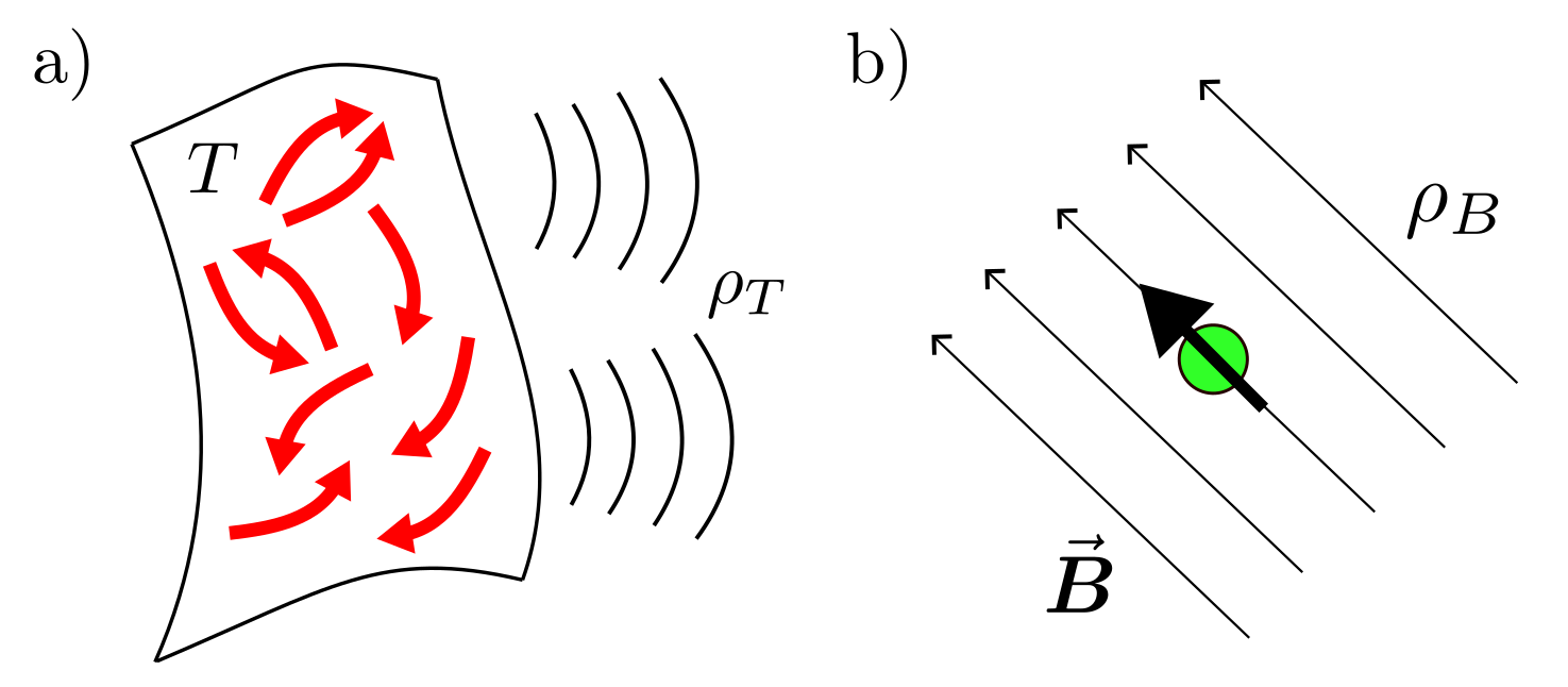
An example of parameter estimation would be receiving the radiation generated by a distribution of currents on a plane, which depends on the properties of the source, like the temperature for example 1. In this scenario, the quantum probe is the radiation. Since the emission of the radiation happens by hypothesis in a far and unaccessible region, we don’t have direct access to the quantum channel that performs the encoding, but only to the encoded states $\rho_T$ , which is the state of the radiated field at detection.

An example of a quantum metrological task is the estimation of the environmental magnetic field with a spin, for which we can choose the initial state and the duration of the interaction. The final state of the spin is $\rho_B$ .

A parameter can be continuous or discrete. Naturally continuous parameters are the magnetic field and the temperature, for example. A discrete parameter is the sign of a signal or the structure of an interaction 2. When discrete parameters are present, we are in the domain of hypothesis testing. In a metrological task, we may have a mix of continuous and discrete parameters, like in the dolinar receiver.

A parameter can be a nuisance; which is an unknown parameter that needs to be estimated, on which we however do not evaluate the precision of the procedure because we are not directly interested in the estimation of this parameter. An example of this is the fluctuating optical visibility of an interferometer when we are only interested in the phase. Estimating the nuisance parameters is often necessary/useful to estimate the parameters of interest. Whether a parameter is a nuisance or not is not specified in the class Parameter, but in the user-defined method loss_function() of the classes StatefulSimulation.

1: E. Köse and D. Braun Phys. Rev. A 107, 032607 (2023).
2: A. A. Gentile, B. Flynn, S. Knauer, et al. Nat. Phys. 17, 837–843 (2021).

Attributes

bounds: Tuple[float, float]

Tuple of extrema of the set of admissible values for the parameter. It is defined both for continuous and discrete parameters. In this latter case it is bounds[0]=min(values) and bounds[1]=max(values).

values: Tuple[float, …]

Tuple of admissible values for a parameter. This tuple contains the values passed to the class constructor in the parameter values, sorted from the smallest to the largest and without repetitions.

Achtung! This attribute is defined only for a discrete parameter.

continuous: bool

Determines if the parameter is continuous or not. It controls the behavior of the reset() method.

randomize: bool

Determines if the initialization of the parameter values is stochastic or deterministic. It controls the behavior of the reset() method.

name: str

Name of the parameter.

bs: int

Size of the first dimension of the Tensor produced by the reset() method and number of estimations performed simultaneously in the simulation.

prec: str

Floating point precision of the parameter values, can be float32 or float64.

Notes

Beside the variables passed to the constructor, a Parameter object requires the manual change of two other attributes to work properly. One attribute is the precision prec, which can be set to either float32 or float64 (with the default value being float64). The other attribute is the batchsize bs, which has a default value of 0. These changes are made automatically if the Parameter object is defined within the call to the constructor of the PhysicalModel class.

Parameters passed to the class constructor.

Parameters

bounds: Tuple[float, float], optional

Tuple of floats containing the extrema of the interval of admissible values for a continuous parameter, where bounds[0] is the minimum and bounds[1] the maximum.

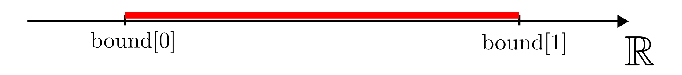
If the bounds parameter is passed to the object constructor, then the Parameter object is automatically treated as continuous and the attribute continuous is therefore set to True.

Achtung! The bounds and values parameters are mutually exclusive and cannot both be both passed to the Parameter class constructor.

values: Tuple[float, …], optional

Tuple of float of unknown length containing the admissible values for a discrete parameter. Repetitions are ignored.

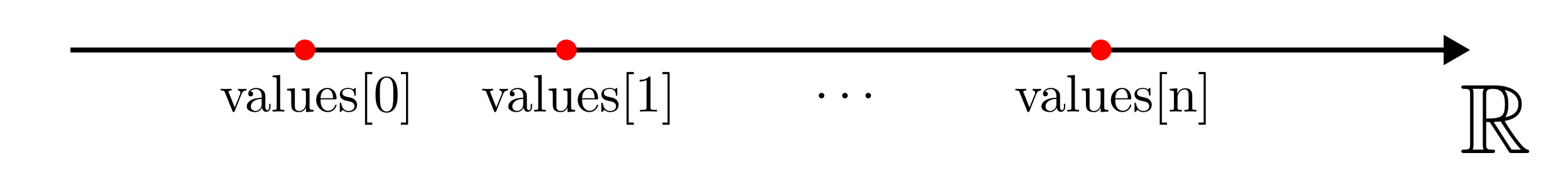
If the values parameter is passed to the constructor of the object, this is automatically treated as a discrete parameter and the attribute continuous is set to False.

Achtung! The bounds and values parameters are mutually exclusive and cannot both be both passed to the Parameter class constructor.

Achtung! Even if only the values parameter is passed in the call to the class constructor, the bounds tuple is still included in the attributes. In this case it is defined as bounds[0]=min(values) and bound[1]=max(values).

randomize: bool = True

This flag controls whether the function reset() should generate random values or behave (almost) deterministically.

Note: The value of this flag should be changed only for a discrete parameter.

Th use of this flag is explained through the following example. Consider a parameter that can assume three values {a, b, c}. If the randomization is on and we call the reset() method with parameter num_particles, we get a Tensor of shape (bs, num_particles, 1) where the entries of each row have been extracted uniformly and stochastically from the set {a, b, c}. For example, if num_particles=12, a row could look like (a, b, a, c, b, b, a, c, a, c, a, b). If we however set randomize=False, then the rows are all equal to (a, a, a, a, b, b, b, b, c, c, c, c). With the randomization turned off, if k>1 is the number of admissible values for the parameter, we have lfloor num_particles/k rfloor repetitions of each element of the tuple values in each row of the output Tensor. If num_particles is not divisible by k, the values of the last, at most k-1, remaining particles are extracted uniformly and stochastically from the tuple values.

If we generate a single particle, its value will always be extracted randomly and uniformly from values, since one will be always the remainder of the division 1/k.

The utility of setting randomize=False is confined to the task of hypothesis testing, where we want a number of particles in the particle filter that matches the number of hypotheses. In this case, in the initialization of the ParticleFilter object, we will set num_particles=k, with k being the number of hypotheses, so that with randomize=False, the particle filter ensemble contains exactly one and only one particle for each hypothesis. The reset() method, called with parameter num_particles=1 for generating the true values in the simulation, returns, however, a single uniformly randomly extracted hypothesis among the admissible ones defined in values.

Note: Setting this flag to False for a continuous parameter has undesired effects. In this scenario the true values of the parameter in the simulation are generated by calling reset() with num_particles=1, which, for a continuous parameter, is implemented as a linspace(bounds[0], bounds[1], 1), that always returns bounds[0].

name: str

Name of the parameter.

reset(seed: Tensor, num_particles: int, fragmentation: int = 1) → Tensor

Generates a Tensor of admissible values for the parameter.

Produces a Tensor of shape (bs, num_particles, 1) of type prec, with a series of independent valid values for the parameter. Valid means that they lie in the interval specified by the tuple bounds if the parameter is continuous or, if it is discrete, that they belong to the tuple values, both being attributes of the Parameter class. The random entries are generated to cover uniformly the set of admissible values, whether it is discrete or continuous. According to the parameter randomize of the class constructor, this function implements a stochastic or deterministic generation of the Tensor entries.

Parameters

seed: Tensor

Seed of the random number generator that initializes the values of the parameter. It is a Tensor of type int32 and of shape (2,).

This is the kind of seed that is accepted by the stateless random functions of the module tensorflow.random.

num_particles: int

Size of the second dimension of the Tensor generated by this method. It is the number of values generated for each batch.

fragmentation: int = 1

Number of pattern repetition in populating the particles with the parameter values. This parameter is only important for a discrete parameter with randomize=False.

Returns

Tensor: Tensor of shape (bs, num_particles, 1) and type prec, where bs is the batch size of the Parameter object, num_particles is passed to the method call, and prec is the floating-point precision (can be either float32 or float64), which is an attribute of the class Parameter.

Notes

This method is used in ParticleFilter to initialize the particle filter ensemble and in PhysicalModel and children classes to produce the true values of the parameter in the estimation task, according to which the outcomes of the measurements are simulated.

Achtung!: This method should be called with randomize=True for a continuous parameter. If randomize=False, the true values of the parameter in the simulation of the estimation are generated by calling this method with num_particles=1, which, for a continuous parameter is implemented as a linspace(bounds[0], bounds[1], 1), which always returns bounds[0].

trim_single_param(old_param: Tensor, param: Parameter, one_arr: Tensor) → Tensor

Trims the values of a given Tensor to be within the bounds set for the corresponding Parameter object. If the parameter is discrete the values of the particles are levelled to the closest element among the admissible values.

Parameters

old_param: Tensor: Tensor of values for the parameter param that do not necessarily lay in the acceptable region of parameter values, defined by param.bounds. The shape and the type of this Tensor must be the same of one_arr.
param: Parameter: Describes abstractly the parameter.
one_arr: Tensor: Tensor filled with ones, of the same type and shape as old_param.

Returns

Tensor: A modified version of old_param, where all the entries that were greater than param.bounds[1] have been set to param.bounds[1] and all those that were smaller than param.bounds[0] have been set to param.bounds[0]. If the parameter is discrete and some entries of old_param don’t exactly belong to the set of admissible values, i.e. param.values, the said entries are “levelled” to the closest element of param.values. This is useful for correcting the distortions of the discrete parameter values introduced by the perturbation in the resampling procedure.

Notes

Since discrete parameters also have a bounds attribute, this function works on them as well. It is used in the resampling routine of the ParticleFilter class, where the particles are perturbed or newly generated and could fall out of the admissible values set.

physical_model

Submodule containing the PhysicalModel class alongside with StateSpecifics and Control.

class Control(name: str, is_discrete: bool = False)

Bases: object

Control parameter for the physical sensor.

A control is a tunable parameter that can be adjusted during the experiment. This could be for example the measurement duration, the detuning of the laser frequency driving a cavity, a tunable phase in an interferometer, or other similar parameters.

In a pictorial sense, control parameters are all the buttons and knobs on the electronics of the experiment.

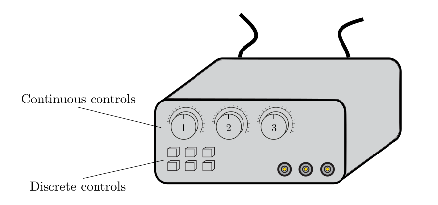
A control can be continuous if it takes values in an interval, or discrete if it takes only a finite set of values (like on and off).

is_discrete: bool = False

If the parameter is discrete this flag is true.

If in the simulation at least one of the controls is discrete, then the control_strategy attribute of the Simulation class should be a callable with header

controls, log_prob_control = control_strategy(input_strategy, rangen)

that is, it can contain stochastic operations (like the extraction of the discrete control from a probability distribution) and it must return the logarithm of the extraction probability of the chosen controls.

name: str: Name of the control.

class PhysicalModel(batchsize: int, controls: List[Control], params: List[Parameter], state_specifics: StateSpecifics, *, recompute_state: bool = True, outcomes_size: int = 1, prec: str = 'float64')

Bases: object

Abstract representation of the physical system used as quantum probe.

This class and its children, StatefulPhysicalModel and StatelessPhysicalModel, contain a description of the physics of the quantum probe, of the unknown parameters to estimate, of the dynamics of their encoding on the probe, and of the measurements.

Achtung! In implementing a class for some particular device, the user should not directly derive PhysicalModel, but instead the classes StatefulPhysicalModel and StatelessPhysicalModel should be the base objects.

When programming the physical model, the first and most important decision to make is whether the model is stateful or stateless. In the former case, StatefulPhysicalModel should be used, while in the latter case StatelessPhysicalModel should be chosen. The probe is stateless if it is reinitialized after each measurement and no classical information needs to be passed from one measurement to the next, other than that contained in the particle filter ensemble. If this is not the case, then the probe is stateful.

Achtung! If some classical information on the measurement outcomes needs to be passed down from measurement to measurement, other than the information contained in the particle filter ensemble, then the probe is stateful. For example, if we perform multiple weak measurements on a signal and want to keep track of the total number of photons observed, then this information is part of the signal state. See the dolinar module for an example.

Attributes

bs: int: The batch size of the physical model, i.e., the number of probes on which the estimation is performed simultaneously in the simulation.
controls: List[Control]: A list of controls on the probe, i.e., the buttons and knobs of the experiment.
params: List[Parameter]: A list of unknown parameters to be estimated, along with the corresponding sets of admissible values.
controls_size: int: The number of controls on the probe, i.e., the length of the controls attribute.
d: int: The number of unknown parameters to estimate, i.e., the length of the params attribute.
state_specifics: StateSpecifics: The size of the last dimension and type of the Tensor used to represent the state of the probe internally in the simulation.
recompute_state: bool: A flag passed to the constructor of the PhysicalModel class; it controls whether the state ensemble should be recomputed after a resampling of the particles or not.
outcomes_size: int: A parameter passed to the constructor of the PhysicalModel class; it is the number of scalar outcomes of a measurement on the probe.
prec: str: The floating point precision of the controls, outcomes, and parameters.

Examples

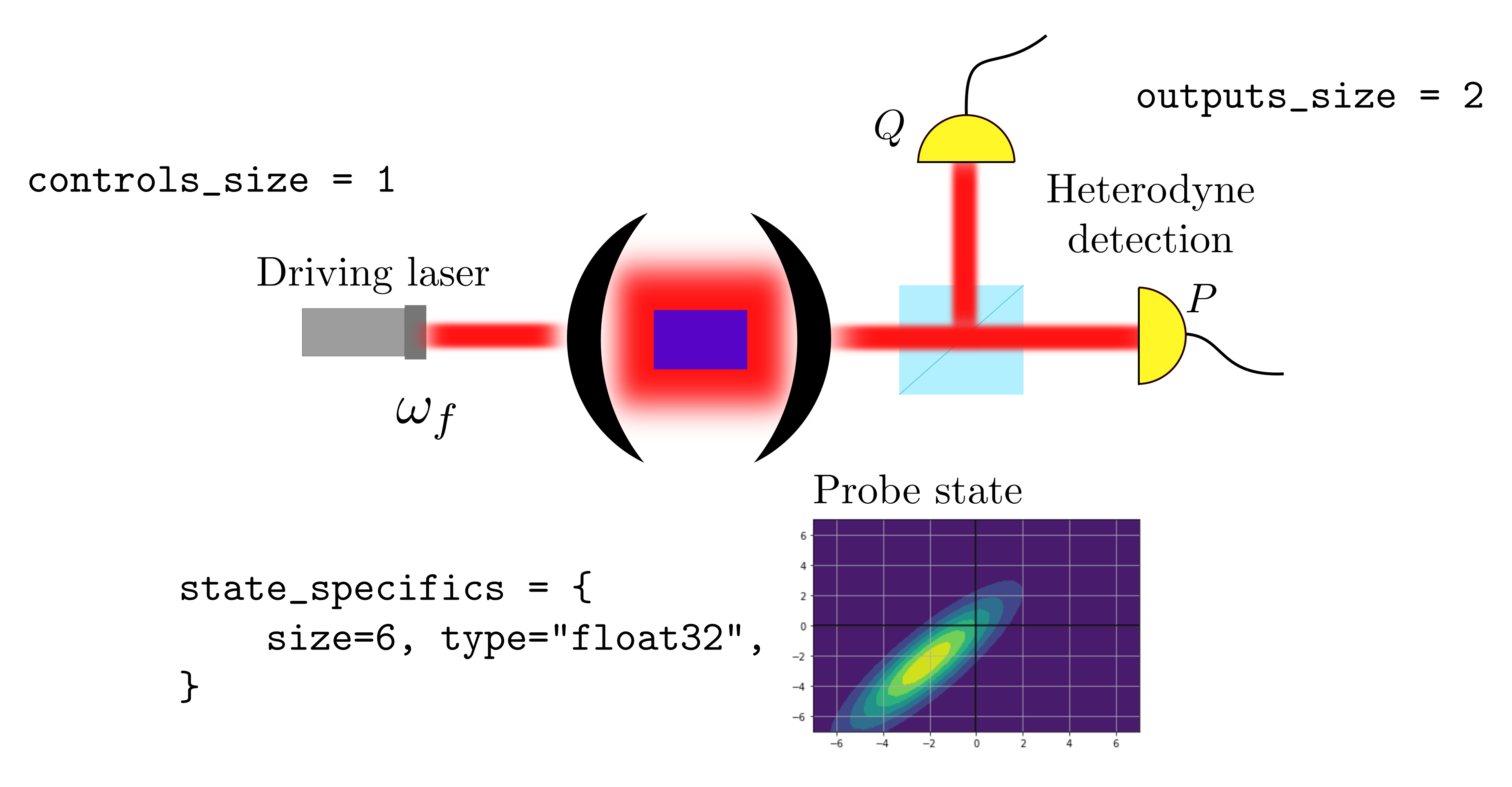
For a metrological task performed on a cavity that is driven by a laser, and where we can control the laser frequency, we have control_size=1. If a heterodyne measurement is performed on the cavity, then outcomes_size=2, because a measurement produces an estimate for both the quadratures. Assuming the cavity state is Gaussian, it can be represented by 6 real numbers (two for the mean and four for the covariance). The number of scalar quantities can be reduced to 5 by observing that the covariance matrix is symmetric.

Parameters passed to the constructor of the PhysicalModel class.

Parameters

batchsize: int

Batch size of the physical model, i.e., the number of simultaneous estimations in the simulation.

controls: List[Control]

A list of controls for the probe (the buttons and knobs of the experiment).

params: List[Parameter]

A list of Parameter objects that represent the unknowns of the estimation.

state_specifics: StateSpecifics

The size of the last dimension and type of the Tensor used to represent internally in the simulation the state of the probe.

recompute_state: bool = True

Controls whether the state ensemble should be recomputed with the method recompute_state() after a resampling of the particles or not.

Achtung! This flag should be deactivated only if the states in the ensemble don’t depend on the particles or if the resampling has been deactivated.

Recomputing the state is very expensive, especially when there have already been many measurement steps. One should consider whether to resample the particles at all in a simulation involving a relatively large quantum state.

outcomes_size: int = 1

Number of scalars collected in a measurement on the probe.

prec: str = “float64”

Floating point precision of the controls, outcomes, and parameters.

count_resources(resources: Tensor, controls: Tensor, true_values: Tensor, meas_step: Tensor) → Tensor

Updates the resource Tensor, which contains, for each estimation in the batch, the amount of resources consumed up to the point this method is called.

Achtung! This method has to be implemented by the user.

The optimization of the estimation precision and the visualization of the performances of an agent are organized within the precision-resources paradigm. The precision is identified with the loss to be minimized in the training cycle, defined in loss_function(), but the precisions of two instances of the same metrological task can only be fairly compared if the costs involved in them is the same. This cost is what we call resource. Some examples of resources are the number of measurements on the probe, the number of identical codified states consumed, the amplitude of a signal, the total measurement time, etc. There is no right or wrong resource in an estimation task, it depends on the user choices and on his understanding of the limitations in the laboratory implementation of the task.

For each measurement, the method count_resources() computes a scalar value based on the controls of the measurement, the measurement step counter, and the true values of the parameter. This scalar is interpreted as the partial resources $r_i$ consumed in the measurement to which the parameters in the call are referring. These partial resources are summed step by step to get the total amount of consumed resources at step $M$ of the measurement loop in execute(), i.e.

(1) $R = \sum_{i=1}^M r_i \; .$

The measurement loop stops when the total amount of consumed resources reaches the value of the attribute max_resources of the class SimulationParameters, set by the user.

The definition of the resources doesn’t only have an impact on the stopping condition of the measurement loop, but it defines how the performances of an agent are visualized. The function performance_evaluation() produces a plot of the mean loss for the estimation task as a function of the consumed resources. Different definitions of the method count_resources() will produce different plots.

Parameters

resources: Tensor: A Tensor of shape (bs, 1) containing the total amount of consumed resources for each estimation in the batch up to the point this method is called.
controls: Tensor: Controls of the last measurement on the probe. It is a Tensor of shape (bs, controls_size) and of type prec, with bs, controls_size, and prec are attributes of the PhysicalModel class.
true_values: Tensor: Contains the true values of the unknown parameters in the simulations. It is a Tensor of shape (bs, 1, d) and type prec, with bs and d being attributes of the PhysicalModel class.
meas_step: Tensor: The index of the current measurement on the probe system. The counting starts from zero. It is a Tensor of shape (bs, 1) and of type int32.

Return

Tensor: Resources consumed in the current measurement step, for each simulation in the batch. It is a Tensor of shape (bs, 1) of type prec.

Examples

For the estimation of a magnetic field with an NV-center, two common choices for the resources are the number of Ramsey measurements, which mean $r_i=1$ , and the employed time, which is $r_i=\tau$ , where $\tau$ is the interaction time between the magnetic field and the probe.

true_values(rangen: Generator) → Tuple[Tensor]

Provides a batch of fresh “true values” for the parameters of the system, from which the measurement is simulated.

Parameters

rangen: Generator: A random number generator from the module tensorflow.random.

Returns

Tensor: Tensor of shape (bs, 1, d), where bs and d are attributes of the PhysicalModel class. For each estimation in the batch, this method produces a single instance of each parameters in the attribute params, extracted uniformly from the allowed values. For doing so the method reset() is called with num_particles=1, for ech parameter.

class StateSpecifics

Bases: TypedDict

Size and type StateSpeof the probe state collected in a single object.

Examples

For a single-qubit probe, the state can be represented by a 2x2 complex matrix with four entries, or by a 3-dimensional vector of real values using the Bloch representation. For a cavity with a single bosonic mode, which is always in a Gaussian state, we need a 2x2 real covariance matrix and a 2-dimensional real vector to represent the state. This requires a total of 6 real values, which can be reduced to 5 noticing that the covariance matrix is symmetric.

size: int: Size of a 1D Tensor necessary to describe unambiguously the state of the probe.

type: str: Type of the Tensor representing the probe state. Can be whatever type admissible in Tensorflow.

stateful_physical_model

Module containing the stateful version of PhysicalModel.

class StatefulPhysicalModel(batchsize: int, controls: List[Control], params: List[Parameter], state_specifics: StateSpecifics, *, recompute_state: bool = True, outcomes_size: int = 1, prec: str = 'float64')

Bases: PhysicalModel

Abstract description of a stateful quantum probe.

Parameters passed to the constructor of the PhysicalModel class.

Parameters

batchsize: int

Batch size of the physical model, i.e., the number of simultaneous estimations in the simulation.

controls: List[Control]

A list of controls for the probe (the buttons and knobs of the experiment).

params: List[Parameter]

A list of Parameter objects that represent the unknowns of the estimation.

state_specifics: StateSpecifics

The size of the last dimension and type of the Tensor used to represent internally in the simulation the state of the probe.

recompute_state: bool = True

Controls whether the state ensemble should be recomputed with the method recompute_state() after a resampling of the particles or not.

Achtung! This flag should be deactivated only if the states in the ensemble don’t depend on the particles or if the resampling has been deactivated.

outcomes_size: int = 1

Number of scalars collected in a measurement on the probe.

prec: str = “float64”

Floating point precision of the controls, outcomes, and parameters.

initialize_state(parameters: Tensor, num_systems: int) → Tensor

Initialization of the probe state.

Achtung! This method must be implemented by the user.

Parameters

parameters: Tensor: Tensor of shape (bs, num_systems, d) and of type prec, where bs, d, and prec are attribute of the Simulation class. These are values for the unknown parameters associated to each of the probe states that must be initialized in this method, be it the “true values” used to simulate the measurement outcomes or the particles in the particle filter ensemble.
num_systems: int: The number of systems to be initialized for each simulation in the batch. This is the size of the second dimension of the Tensor that this method should return.

Returns

state: Tensor: The initialized state of the probe and/or some classical variable state. This is a Tensor of shape (bs, num_systems, state_specifics[“size”]) of type state_specifics[“type”], where state_specifics is an attribute of the PhysicalModel class. It may be desirable to initialize the state of the probe depending on the values of parameters, for example because the encoding has happened outside of the laboratory and we are given the encoded probe state only. However, if the encoding happens in the lab between the measurements it make sense to reset the probe state at the beginning of the estimation with a parameter independent state.

model(outcomes: Tensor, controls: Tensor, parameters: Tensor, state: Tensor, meas_step: Tensor, num_systems: int = 1) → Tuple[Tensor, Tensor]

Description of the encoding and the measurement on the probe. This method returns the probability of observing a certain outcome and the corresponding evolved state after the measurement backreaction.

Achtung! This method must be implemented by the user.

Achtung! This method does not implement any stochastic evolution. All stochastic operations in the measurement of the probe and in the evolution of the state should be defined in the method perform_measurement().

Suppose that the state of the probe after the encoding is $\rho_{\vec{\theta}, x}$ , where $\vec{\theta}$ is parameter and $x$ is control. The probe state will, in general, depend on the entire history of past outcomes and controls, but we neglect the corresponding subscripts to avoid making the notation too cumbersome. The probe measurement is associated with an ensemble of positive operators $\lbrace M_y^x \rbrace_{y \in Y}$ , where $y$ is the outcome and $Y$ is the set of possible outcomes. According to the laws of quantum mechanics, the probability of observing the outcome $y$ is then

(2) $P(y|\vec{\theta}, x) := \text{tr} \left( M_y^x \rho_{\vec{\theta}, x} \right) \; ,$

and the backreaction on the probe state after having observed $y$ is

(3) $\rho_{\vec{\theta}, x}' = \frac{M_{y}^{x} \rho_{\vec{\theta}, x} M_{y}^{x \dagger}}{\text{tr} \left[ M_{y}^{x} \rho_{\vec{\theta}, x} M_{y}^{x \dagger} \right]} \; .$

Parameters

outcomes: Tensor: Measurement outcomes. It is a Tensor of shape (batchsize, num_systems, outcomes_size) of type prec, where bs and outcomes_size are attributes of the PhysicalModel class.
controls: Tensor: Contains the controls for the measurement. This is a Tensor of shape (bs, num_systems, controls_size) and type prec, where bs and controls_size are attributes of the PhysicalModel class.
parameters: Tensor: Values of the unknown parameters. It is a Tensor of shape (bs, num_systems, d) and type prec, where bs and d are attributes of the PhysicalModel class.
state: Tensor: Current state of the quantum probe, computed from the evolution determined (among other factors) by the encoding of parameters. This is a Tensor of shape (bs, num_systems, state_specifics[“size”]), where state_specifics is an attribute of the PhysicalModel class. Its type is state_specifics[“type”].
meas_step: Tensors: The index of the current measurement on the probe system. The Counting starts from zero. This is a Tensor of shape (bs, num_systems, 1) and of type int32.

Returns

prob: Tensor: Probability of observing the given vector of outcomes, having done a measurement with the given controls, parameters, and states. It is a Tensor of shape (bs, num_systems) and type prec. bs and prec are attributes of the PhysicalModel class.
state: Tensor: State of the probe after the encoding of parameters and the application of the measurement backreaction, associated with the observation of the given outcomes. This is a Tensor of shape (bs, num_systems, state_specifics[“size”]), where state_specifics is an attribute of the PhysicalModel class.

perform_measurement(controls: Tensor, parameters: Tensor, true_state: Tensor, meas_step: Tensor, rangen: Generator) → Tuple[Tensor, Tensor, Tensor]

Performs the stochastic extraction of measurement outcomes and updates the state of the probe.

Achtung! This method must be implemented by the user.

Samples measurement outcomes to simulate the experiment and returns them, together with the likelihood of obtaining such outcomes and the evolved state of the probe after the measurement. Typically, this function contains at least one call to the model() method, which produces the probabilities for the outcome sampling.

Achtung! When using the StatefulPhysicalModel class in combination with BoundSimulation the method perform_measurement() can be implemented to return an outcome extracted from an arbitrary probability distribution, which can be different from the one predicted by the true model of the system. This is used to introduce an importance sampling on the probe trajectories. The log_prob outcome should be the log-likelihood of the outcome according to the modified distribution, while true_state remains the state of the system conditioned on the observation of the outcome. It is important that model implement the true probability. This feature should be used together with the activation of the flag importance_sampling in the constructor of the BoundSimulation object, and should not be used for a Bayesian estimation carried out with the Simulation class.

Parameters

controls: Tensor: Contains the controls for the current measurement. This is a Tensor of shape (bs, 1, controls_size) and type prec, where bs and controls_size are attributes of the PhysicalModel class.
parameters: Tensor: Contains the true values of the unknown parameters in the simulations. The observed measurement outcomes must be simulated according to them. It is a Tensor of shape (bs, 1, d) and type prec, where bs and d are attributes of the PhysicalModel class. In the estimation, these values are not observable, only their effects through the measurement outcomes are.
true_states: Tensor: The true state of the probe in the estimation, computed from the evolution determined (among other factors) by the encoding of the parameter true_values. Like true_values, this information is not observable. This is a Tensor of shape (bs, 1, state_specifics[“size”]), where state_specifics is an attribute of the PhysicalModel class. Its type is state_specifics[“type”].
meas_step: Tensor: The index of the current measurement on the probe system. The counting starts from zero. This is a Tensor of shape (bs, 1, 1) and of type int32.
rangen: Generator: A random number generator from the module tensorflow.random.

Returns

outcomes: Tensor: The observed outcomes of the measurement. This is a Tensor of shape (bs, 1, outcomes_size) and of type prec. bs, outcomes_size, and prec are attributes of the PhysicalModel class.
log_prob: Tensor: The logarithm of the probabilities of the observed outcomes. This is a Tensor of shape (bs, 1) and of type prec. bs and prec are attributes of the PhysicalModel class.
true_state: Tensor: The true state of the probe, encoded with the parameters true_values, after the measurement backreaction corresponding to outcomes is applied. This is a Tensor of shape (bs, 1, state_specifics[“size”]), where state_specifics is an attribute of the PhysicalModel class. Its type is state_specifics[“type”].

stateless_physical_model

Module containing the stateless version of PhysicalModel.

class StatelessPhysicalModel(batchsize: int, controls: List[Control], params: List[Parameter], outcomes_size: int = 1, prec: str = 'float64')

Bases: PhysicalModel

Abstract description of a stateless quantum probe.

Constructor of the StatelessPhysicalModel class.

Parameters

batchsize: int: Batch size of the physical model, i.e., the number of simultaneous estimations in the simulation.
controls: List[Control]: A list of controls for the probe (the buttons and knobs of the experiment).
params: List[Parameter]: A list of Parameter objects that represent the unknowns of the estimation.
outcomes_size: int = 1: Number of scalars collected in a measurement on the probe.
prec: str = “float64”: Floating point precision of the controls, outcomes, and parameters. Can be either “float32” or “float64”.

model(outcomes: Tensor, controls: Tensor, parameters: Tensor, meas_step: Tensor, num_systems: int = 1) → Tensor

Description of the encoding and the measurement on the probe. This method returns the probability of observing a certain outcome after a measurement.

Achtung! This method must be implemented by the user.

Achtung! This method does not implement any stochastic evolution. The stochastic extraction of the outcomes should be defined in the method perform_measurement().

Suppose that the state of the probe after the encoding is $\rho_{\vec{\theta}, x}$ , where $\vec{\theta}$ is parameter and $x$ is control. The probe measurement is associated with an ensemble of positive operators $\lbrace M_y^x \rbrace_{y \in Y}$ , where $y$ is the outcome and $Y$ is the set of possible outcomes. According to the laws of quantum mechanics, the probability of observing the outcome $y$ is then

(4) $P(y|\vec{\theta}, x) := \text{tr} \left( M_y^x \rho_{\vec{\theta}, x} \right) \; .$

Parameters

outcomes: Tensor: Measurement outcomes. It is a Tensor of shape (bs, num_systems, outcomes_size) of type prec, where bs, outcomes_size, and prec are attributes of the PhysicalModel class.
controls: Tensor: Contains the controls for the measurement. This is a Tensor of shape (bs, num_systems, controls_size) and type prec, where bs, controls_size, and prec are attributes of the PhysicalModel class.
parameters: Tensor: Values of the unknown parameters. It is a Tensor of shape (bs, num_systems, d) and type prec, where bs, d, and prec are attributes of the PhysicalModel class.
meas_step: Tensors: The index of the current measurement of the probe system. The counting starts from zero. This is a Tensor of shape (bs, num_systems, 1) and of type int32.

Returns

prob: Tensor: Probability of observing the given outcomes vector, having done a measurement with the given controls and parameters. It is a Tensor of shape (bs, num_systems) and of type prec. bs and prec are attributes of the PhysicalModel class.

perform_measurement(controls: Tensor, parameters: Tensor, meas_step: float, rangen: Generator) → Tuple[Tensor, Tensor]

Performs the stochastic extraction of measurement outcomes.

Achtung! This method must be implemented by the user.

Samples measurement outcomes to simulate the experiment and returns them, together with the likelihood of obtaining such outcomes. Typically, this function contains at least one call to the model() method, which produces the probabilities for the outcome sampling.

Parameters

controls: Tensor: Contains the controls for the current measurement. This is a Tensor of shape (bs, 1, controls_size) and type prec, where bs and controls_size are attributes of the PhysicalModel class.
parameters: Tensor: Contains the true values of the unknown parameters in the simulations. The observed measurement outcomes must be simulated according to them. It is a Tensor of shape (bs, 1, d) and type prec, where bs and d are attributes of the PhysicalModel class. In the estimation, these values are not observable, only their effects through the measurement outcomes are.
meas_step: Tensor: The index of the current measurement on the probe system. The counting starts from zero. This is a Tensor of shape (bs, 1, 1) and of type int32.
rangen: Generator: A random number generator from the module tensorflow.random.

Returns

outcomes: Tensor: The observed outcomes of the measurement. This is a Tensor of shape (bs, 1, outcomes_size) and of type prec. bs, outcomes_size, and prec are attributes of the PhysicalModel class.
log_prob: Tensor: The logarithm of the probabilities of the observed outcomes. This is a Tensor of shape (bs, 1) and of type prec. bs and prec are attributes of the PhysicalModel class.

particle_filter

Submodule containing the class ParticleFilter necessary for Bayesian estimation.

class ParticleFilter(num_particles: int, phys_model: PhysicalModel, resampling_allowed: bool = True, resample_threshold: float = 0.5, resample_fraction: Optional[float] = None, alpha: float = 0.5, beta: float = 0.98, gamma: float = 1.0, scibior_trick: bool = True, trim: bool = True, prec: str = 'float64')

Bases: object

Particle filter object, with methods to reset the particle ensemble and perform Bayesian filtering for quantum metrology.

Given the tuple of unknown parameters $\vec \theta=(\theta_1, \theta_2, \cdots, \theta_d)$ , in the Bayesian framework we start from a prior $p(\theta)$ and update it after each observation through the Bayes rule. In simulating such procedure (called Bayesian filtering) we need a computer representation of a generic probability distribution on the parameters. We can approximate a distribution $p(\theta)$ with a weighted sum of delta functions as follows:

(5) $p(\vec \theta) = \sum_{j=1}^{N} w_j \delta(\vec \theta - \vec \theta_j),$

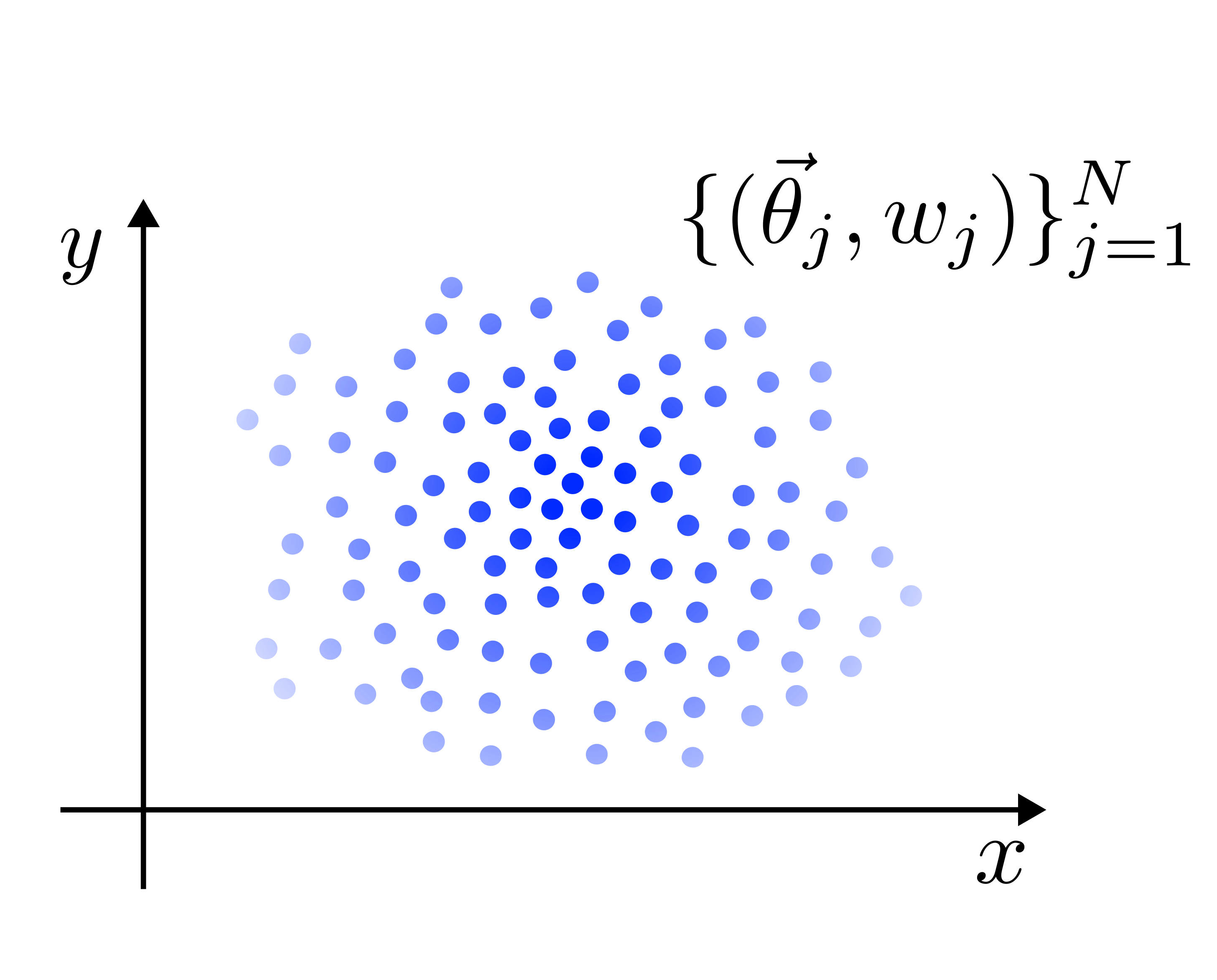
where the vectors $\vec \theta_j$ are called particles, while the real numbers $w_i$ are the weights. The integer $N$ is the attribute np of the ParticleFilter object. The core idea is that the posterior distribution is represented by an ensemble of particles and weights $\lbrace (\vec \theta_j, w_j) \rbrace_{j=1}^N$ . The Bayesian filtering techniques that use this kind of representations for the posterior are called particle filter methods.

In the figure, we represent the ensemble of a two-dimensional particle filter, where the intensity of the color is proportional to the weight associated with each particle.

The update of the posterior in the particle filter becomes the update of the weights $w_i$ .

Attributes

bs: int

Batchsize of the particle filter, i.e. number of Bayesian estimations performed simultaneously.

np: int

Parameter num_particles passed to the constructor of the class. It is the number of particles in the ensemble.

phys_model: PhysicalModel

Abstract description of the physical model of the quantum probe passed to the ParticleFilter constructor. It also contains the description of the parameters to estimate, on the basis of which the particles of the ensemble are initialized.

resampling: bool

Flag resampling_allowed passed to the constructor of ParticleFilter.

Achtung! This attribute has no effect inside the methods of the ParticleFilter. Calling the method full_resampling() will resample the particles if needed also with resampling=False.

state_size: int

Size of the state of the probe, it is phys_model.state_specifics[“size”], where phys_model is the attribute of ParticleFilter.

state_type: str

Type of the state vector of the probe, it is phys_model.state_specifics[“type”], where phys_model is the attribute of ParticleFilter.

d: int

Number of unknown parameters of the simulation, it is the length of the attribute params.

prec: str

Floating point precision of the parameter values. Can be either float32 or float64. It is the parameter prec passed to the constructor.

Notes

This class can deal with a whole batch of particle filter ensembles that are updated simultaneously. The batchsize attribute bs is taken from phys_model in the initialization.

This implementation of the particle filter is fully differentiable and can, therefore, be used in the training loop of a neural network agent that controls the experiment. It is trivial to see that the Bayes update is differentiable, while the differentiability of the resampling 3 is achieved through a combination of soft resampling 4 and the method of Ścibior and Wood 5.

Constructor of the ParticleFilter class.

Parameters

num_particles: int

Number of particles in the ensemble of the particle filter.

phys_model: PhysicalModel

Contains the physics of the quantum probe and the methods to operate on its state and compute the probabilities of observing a certain outcome in a measurement. This object is used in the apply_measurement() method, which performs the Bayesian update on the particle weights.

resampling_allowed: bool = True

Controls whether the resampling is allowed or not for a particular instance of ParticleFilter. The typical case in which we set resampling_flag=False is that of hypothesis testing, where we have a single discrete parameter and num_particles equals the number of hypotheses.

This flag isn’t used directly in this class, but in the StatelessSimulation and StatefulSimulation classes, which use the methods of ParticleFilter.

resample_threshold: float = 0.5

The method full_resampling() verifies the need for resampling for a certain particle filter ensemble according to the effective particle number, defined as

(6) $N_{\text{eff}} := \frac{1}{\sum_{j=1}^N w_j^2} \; .$

Indicating with $r_t$ the resample_threshold, the particle filter identifies an ensemble as in need of resampling when $N_{\text{eff}}<r_t N$ .

resample_fraction: float = 0.98

The method full_resampling() triggers the resampling for the whole batch of particle filter ensembles if at least a fraction resample_fraction of simulations are in need of resampling. Also those simulations in the batch that don’t need resampling will be resampled.

alpha: float = 0.5

In the method resample() an importance sampling of the particles is performed, where the extraction is done from a distribution, being the one defined by the ensemble mixed with a uniform distribution on the particles. This procedure, called soft resampling, aims to make the update step differentiable. The mixing coefficient is the parameter alpha, and it is indicated with $\alpha$ in the equations.

This parameter quantitatively controls the flow of derivatives through the resampling routine and the effectiveness of the resampling. With alpha=1, regular resampling without mixing occurs, but no derivatives can flow through this operation. With alpha=0, differentiability is achieved, but no resampling is done. There is a tradeoff between the efficiency of the soft resampling and its differentiability.

beta: float = 0.98

In the method resample(), a Gaussian perturbation of the particles obtained from the soft resampling is performed. The intensity of this perturbation is controlled by the parameter 1.0-beta, which is indicated by $\beta$ in the equations.

gamma: float = 1.0

This parameter controls the fraction of num_particles that are extracted in the soft resampling. The remaining fraction of particles, 1.0-gamma, are newly generated from a Gaussian distribution having the same mean and variance as the posterior distribution before the resampling. This parameter, like alpha and beta, regulates the behavior of the resample() method and is indicated by $\gamma$ in the equations.

Achtung! Proposing new particles during a resampling won’t work when one ore more discrete parameters are present. The advice in these cases is to keep gamma=1.0.

scibior_trick: bool = True

This flag controls the use of the method proposed by Ścibior and Wood to make the resampling differentiable. It can be used alone or together with soft resampling to improve the flow of the gradient through the particle ensemble resampling steps.

trim: bool = True

After the Gaussian perturbation of the particles or their extraction from scratch from a Gaussian, they may fall outside the admissible bounds for the parameters. If trim=True, they are cast again inside the bounds using the function trim_single_param().

prec: str = “float64”

This parameter indicates the floating-point precision of the particles and weights, it can be either float64 or float32.

3

1. Granade et al, New J. Phys. 14 103013 (2012).

4

Ma, P. Karkus, D. Hsu, and W. S. Lee, arXiv:1905.12885 (2019).

5

Ścibior, F. Wood, arXiv:2106.10314 (2021).

apply_measurement(weights: Tensor, particles: Tensor, state_ensemble: Tensor, outcomes: Tensor, controls: Tensor, meas_step: Tensor) → Tuple[Tensor, Tensor]

Bayesian update of the weights of the particle filter.

Consider $x$ the outcome of the last observation on the probe and $y$ the control. The weights are updated as

(7) $w_j \leftarrow \frac{p(x|\vec{\theta}_j, y, \rho_j) w_j}{\sum_{j=1}^N p(x|\vec{\theta}_j, y, \rho_j) w_j} \; ,$

where $p(x|\vec{\theta}_j, y, \rho_j)$ is the probability of observing the outcome $x$ under the control $y$ , and $\vec{\theta}_j$ the j-th particles with its associated state $\rho_j$ before the encoding and the measurement.

Parameters

weights: Tensor: A Tensor of weights with shape (bs, np) and type prec. bs, np, and prec are attributes of the ParticleFilter class.
particles: Tensor: A Tensor of particles with shape (bs, np, d) and type prec. bs, np, d, and prec are attributes of the ParticleFilter class.
state_ensemble: Tensor: The state of the probe system before the last measurement for each particle. It is a Tensor of shape (bs, np, state_size) and of type state_type. Here, state_size and state_type are attributes of ParticleFilter. In the Bayes rule formula, the state_ensemble is indicated with $\rho_j$ .
outcomes: Tensor: The outcomes of the last measurement on the probe. It is a Tensor of shape (bs, phys_model.outcomes_size) and of type prec. In the Bayes rule formula, it is indicated with $x$ .
controls: Tensor: The controls of the last measurement on the probe. It is a Tensor of shape (bs, phys_model.controls_size) and of type prec. In the Bayes rule formula, it is indicated with $y$ .
meas_step: Tensor: The index of the current measurement on the probe system. The counting starts from zero. It is a Tensor of shape (bs, 1) and of type int32.

Returns

weights: Tensor: Updated weights after the application of the Bayes rule. It is a Tensor of shape (bs, np) and of type prec. bs, np, and prec are attributes of the ParticleFilter class.
state_ensemble: Tensor: Probe state associated to each particle after the measurement backreaction associated to outcomes. It is a Tensor of shape (bs, np, state_size) and of type state_type. bs, np, state_size, and state_type are attributes of the ParticleFilter class.

Notes

If an outcome is observed that is not compatible with any of the particles, this method ignores the measurements for the corresponding batch element. Such observation is treated as an outlier.

check_resampling(weights: Tensor, count_for_resampling: Tensor) → Tensor

Checks the resampling condition on the effective number of particles for each simulation in the batch.

A particle filter ensemble is in need of resampling when the effective number of particles, defined in Eq.6, is less then a fraction resample_threshold of the total particle number.

Parameters

weights: Tensor: Tensor of weights of shape (bs, np) and of type prec. bs, np, and prec are attributes of the ParticleFilter class.
count_for_resampling: Tensor: Tensor of bool of shape (bs, 1), that says whether a certain ensemble in the batch should be counted or not in the total number of active simulation. Some estimations in the batch may have already terminated and are not to be counted in assessing the need of launching the resampling routine. If a fraction resample_fraction of the active simulations needs resampling then the whole batch is resampled.

Returns

trigger_resampling: Tensor: Tensor of shape (bs, ) and of type bool that indicates whether the corresponding batch element should undergo resampling or not.

compute_covariance(weights: Tensor, particles: Tensor, batchsize: Optional[Tensor] = None, dims: Optional[int] = None) → Tensor

Computes the covariance matrix of the Bayesian posterior distribution.

The empirical covariance matrix of the particle filter ensemble is defined as:

(8) $\Sigma = \sum_{j=1}^N w_j^t (\vec{\theta}_j - \vec{\mu}) (\vec{\theta}_j - \vec{\mu})^\intercal,$

where $\vec{\mu}$ is the mean value returned by the method compute_mean().

Parameters

weights: Tensor: A Tensor of weights of shape (bs, np) and of type prec. bs, np, and prec are attributes of the ParticleFilter class.
particles: Tensor: A Tensor of particles of shape (bs, np, d) and of type prec, bs, np, d, and prec are attributes of the ParticleFilter class.
dims: int, optional: This method can deal with a last dimension for the particles parameter different from the attribute d of the ParticleFilter object. If this optional parameter is passed to the method call, then the shape of particles is expected to be (bs, np, dims). Its typical use is when we compute the covariance of a subset only of the parameters.

Returns

Tensor: A Tensor of shape (bs, d, d) of type prec with the covariance matrix of the Bayesian posterior for each ensemble in the batch. if dims was passed to the function call then the outcome Tensor has shape (bs, dims, dims).

compute_max_weights(weights: Tensor, particles: Tensor) → Tensor

Returns the particle with the maximum weight in the ensemble.

Achtung! This method does not return the true maximum of the posterior if the particles are not equidistant in the parameter space. In general, it should not be used if the resampling is active or if the initialization of the particles in the ensemble is stochastic. Its use case is for pure hypothesis testing, where it returns the most plausible hypothesis.

Parameters

weights: Tensor: A Tensor of weights with shape (bs, np) and type prec.
particles: Tensor: A Tensor of particles with shape (bs, np, d) and type prec. Here, d is the attribute of the ParticleFilter object.

Returns

Tensor: A Tensor of shape (bs, d) and type prec with the particle having the highest weight for each ensemble in the batch.

compute_mean(weights: Tensor, particles: Tensor, batchsize: Optional[Tensor] = None, dims: Optional[int] = None) → Tensor

Computes the empirical mean of the unknown parameters based on the particle filter posterior distribution.

The mean $\vec{\mu}$ is computed as follows:

(9) $\vec{\mu} = \sum_{j=1}^N w_j \vec{\theta}_j \; ,$

$w_j$ are the weights of the particles, and $\vec{\theta}_j$ are the particles.

Parameters

weights: Tensor: A Tensor of weights with shape (bs, np) and type prec.
particles: Tensor: A Tensor of particles with shape (bs, np, d) and type prec, where d is the attribute of the ParticleFilter object.
dims: int, optional: This method can handle a particles parameter with a last dimension different from the attribute d of the ParticleFilter class. If dims is passed to the method call, the shape of particles is expected to be (bs, np, dims). This parameter is typically used when computing the mean of a subset of the parameters.

Returns

Tensor: The mean of the unknown parameters computed on the posterior distribution represented by weights and particles. It is a Tensor of shape (bs, d), or possibly (bs, dims) if dims is defined. Its type is prec.

compute_state_mean(weights: Tensor, state_ensemble: Tensor, batchsize: Tensor) → Tensor

Compute the mean state of a particle filter ensemble.

Given the weight $w_j$ and state $\rho_j$ of the j-th particle in the ensemble, the mean state is defined as:

(10) $\bar{\rho} = \sum_{j=1}^N w_j \rho_j.$

Parameters

weights: Tensor: Tensor of particle weights with shape (bs, np) and type prec.
state: Tensor: Tensor of states for the probe, with shape (bs, np, state_size) and type state_type.

Returns

Tensor: Mean state for each estimation in the batch computed with the posterior distribution. It is a Tensor of shape (bs, state_size) and type state_type. state_size and state_type are attributes of the ParticleFilter class.

extract_particles(weights: Tensor, particles: Tensor, num_extractions: int, rangen: Generator) → Tensor

Extracts num_extractions particles from the posterior distribution represented by the particle filter ensemble.

Parameters

weights: Tensor: A Tensor of weights with shape (bs, np) and type prec.
particles: Tensor: A Tensor of particles with shape (bs, np, d) and type prec. Here, d is the attribute of the ParticleFilter object.
num_extraction: int: The number of particles to be stochastically extracted.
rangen: Generator: A random number generator from the module tensorflow.random.

Returns

Tensor: A Tensor of shape (bs, num_extractions, d), of type prec, containing the num_extraction particles sampled from the posterior distribution.

full_resampling(weights: Tensor, particles: Tensor, count_for_resampling: Tensor, rangen: Generator) → Tuple[Tensor, Tensor, Tensor]

Checks the resampling condition on the effective number of particles and applies the resampling if needed.

A particle filter ensemble is in need of resampling when the effective number of particles, defined in Eq.6, is less then a fraction resample_threshold of the total particle number. The whole batch of particle filters gets resampled if at least a fraction resample_fraction of the active simulations, defined by count_for_resampling, is in need of resampling.

Parameters

weights: Tensor: Tensor of weights of shape (bs, np) and of type prec. bs, np, and prec are attributes of the ParticleFilter class.
particles: Tensor: Tensor of particles of shape (bs, np, d) and of type prec. bs, np, d, and prec are attributes of the ParticleFilter class. d is the attribute of ParticleFilter.
count_for_resampling: Tensor: Tensor of bool of shape (bs, 1), that says whether a certain ensemble in the batch should be counted or not in the total number of active simulation. Some estimations in the batch may have already terminated and are not to be counted in assessing the need of launching the resampling routine. If a fraction resample_fraction of the active simulations needs resampling then the whole batch is resampled.
rangen: Generator: Random number generator from the module tensorflow.random.

Returns

weights: Tensor: Resampled weights. Tensor of shape (bs, np) and of type prec. bs, np, and prec are attributes of the ParticleFilter class.
particles: Tensor: Resampled particles. Tensor of shape (bs, np, d) and of type prec. bs, np, d, and prec are attributes of the ParticleFilter class.
resample_flag: Tensor: Tensor of shape (, ) of type bool that informs whether the resampling has been executed or not.

partial_resampling(weights: Tensor, particles: Tensor, count_for_resampling: Tensor, rangen: Generator) → Tuple[Tensor, Tensor, Tensor]

Checks the resampling condition on the effective number of particles and applies the resampling if needed.

Parameters

weights: Tensor: Tensor of weights of shape (bs, np) and of type prec. bs, np, and prec are attributes of the ParticleFilter class.
particles: Tensor: Tensor of particles of shape (bs, np, d) and of type prec. bs, np, d, and prec are attributes of the ParticleFilter class. d is the attribute of ParticleFilter.
count_for_resampling: Tensor: Tensor of bool of shape (bs, 1), that says whether a certain ensemble in the batch should be counted or not in the total number of active simulation. Some estimations in the batch may have already terminated and are not to be counted in assessing the need of launching the resampling routine. If a fraction resample_fraction of the active simulations needs resampling then the whole batch is resampled.
rangen: Generator: Random number generator from the module tensorflow.random.

Returns

weights: Tensor: Resampled weights. Tensor of shape (bs, np) and of type prec. bs, np, and prec are attributes of the ParticleFilter class.
particles: Tensor: Resampled particles. Tensor of shape (bs, np, d) and of type prec. bs, np, d, and prec are attributes of the ParticleFilter class.

recompute_state(index: Tensor, particles: Tensor, hist_control_rec: Tensor, hist_outcomes_rec: Tensor, hist_continue_rec: Tensor, hist_step_rec: Tensor, num_steps: int) → Tensor

Routine that recomputes the state ensemble starting from the measurement outcomes and the controls.

When a resampling of the particle filter ensemble is carried out, a new set of particles is produced. In this situation state_ensemble generated by initialize_state() and updated in the measurement loop inside the method execute() still refers to the old particles. The only way to align the state ensemble with the new particles is to re-initialise and re-evolve the state ensemble with the applied controls, the observed outcomes, and the new particles. That is the role of this method.

Parameters

index: Tensor: Tensor of shape (,) and type int32 that contains the number of iterations of the measurement loop in execute(), as this method is called.
particles: Tensor: Tensor of particles of shape (bs, np, d) and of type prec. d is an attribute of ParticleFilter.
hist_outcomes_rec: Tensor: Tensor of shape (num_step, bs, phys_model.outcomes_size) and of type prec. It contains the history of the outcomes of the measurements for all the estimations in the batch up to the point at which this method is called. It is generated automatically in the execute() method.
hist_control_rec: Tensor: Tensor of shape (num_steps, bs, phys_model.control_size) and of type prec. It contains the history of the controls of the measurements for all the estimations in the batch up to the point at which this method is called. It is generated automatically in the execute() method.
hist_step_rec: Tensor: Tensor of shape (num_steps, bs, 1) that contains, for each loop of the measurement cycle, the index of the last measurement performed on each estimation in the batch. Different estimations can terminate with a different number of total measurements performed. This Tensor is fundamentally a table that shows for each loop of the measurement cycle (row index) the number of measurements performed up to that point for each estimation (column index). Because for some loops the measurement might be applied only to a subset of estimations, some cells can show a number of measurements lower than the current number of completed loops in the measurement cycle. This Tensor is generated automatically in the execute() method.
hist_continue_rec: Tensor: A Tensor of shape (num_steps, bs, 1) and type int32, hist_continue_rec is a flag Tensor indicating whether a simulation in the batch is ended or not. This flag is necessary because different simulations may stop at different numbers of measurements. The typical column of hist_continue_rec consists of a series of contiguous ones, say in number of M, followed by zeros until the end of the row. This tells us that the particular simulation to which the row refers, consisted of M measurements so far. In recomputing the state with different values for the particles, M measurement should be performed for that particular simulation. The parameter hist_continue_rec is generated automatically in the Simulation.execute method and could be easily derived from hist_step_rec, which contains more information.
batchsize: Tensor: Dynamical batchsize of the recomputed states.
num_steps: int: The maximum number of steps in the training loop. It is the attribute num_steps of the data class SimulationParameters.

Returns

state_ensemble: Tensor: The state of the quantum probe associated with each entry of particles, that has been recomputed using the applied controls and the observed outcomes. Each entry of state_ensemble is the state of the probe computed as if the true values of the parameters were the particles of the ensemble. When these are resampled, the states do not refer anymore to the correct values of the parameters, and the only way to realign them is to recompute them from scratch. state_ensemble is a Tensor of shape (bs, np, state_size) and type state_type, where state_size and state_type are attributes of ParticleFilter.

Notes

The stopping condition in the measurement loop, which determines the number of measurements for an estimation, depends on the number of computed resources, which depends only on the applied controls and observed outcomes. For this reason, it is possible to reuse the objects hist_step_rec and hist_continue_rec, which were generated before the resampling. For the same reason, these objects are actually superfluous in the function call, as they could be recomputed from the hist_outcomes_rec and hist_continue_rec parameters.

resample(weights: Tensor, particles: Tensor, rangen: Generator, batchsize: Optional[Tensor] = None) → Tuple[Tensor, Tensor]

Resample routine of the particle filter.

The resampling procedure works in three steps. First, we mix the probability distribution on the particles represented by the weights $w_j$ with a uniform distribution and construct the soft-weights $q_j$ defined as:

(11) $q_j = \alpha w_j + (1-\alpha) \frac{1}{N} \; ,$

The new particles $\vec{\theta}_j'$ are resampled from the ensemble $\lbrace \vec{\theta}_j, q_j \rbrace$ and the new weight associated with each resampled particle is:

(12) $w_j' \propto \frac{w_{\phi(j)}}{\alpha w_{\phi(j)} + (1-\alpha)\frac{1}{N}} \; ,$

where $\phi(j)$ is the original index in the old ensemble of the j-th particle in the new ensemble. The function $\phi$ is in general neither injective nor surjective. Only a fraction gamma of the total particles np is resampled in this way, and their weights are normalized such that they sum to gamma, i.e.

(13) $\sum_{j=1}^{\gamma N} w_j' = \gamma \; .$

The second step is to perturb the newly extracted particles $\vec{\theta}_j'$ as follows:

(14) $\vec{\theta}_j'' = \beta \vec{\theta}_j' + (1-\beta) \vec{\mu} + \vec{\delta} \; ,$

where $\vec{\mu}$ is the mean value of the parameters calculated from the ensemble before the resampling with the method compute_mean(), and $\vec{\delta}$ is a random variable extracted from a Gaussian distribution, i.e.

(15) $\vec{\delta} \sim \mathcal{N} (0, (1-\beta^2) \Sigma) \; ,$

with $\Sigma$ being the covariance matrix of the ensemble, computed with the method compute_covariance(). The third and last step of the resampling routine is to propose new particles. These are again extracted from a Gaussian distribution, i.e.

(16) $\vec{\theta}_j'' \sim \mathcal{N}(\vec{\mu}, \Sigma) \; .$

A number $(1-\gamma)N$ of particles are sampled in this way with $N$ being the total number of particles np. Their weights are uniform and normalized to $1-\gamma$ , so that together with the particles produced in the first two steps, their weights sum to one.

Parameters

weights: Tensor: Tensor of weights of shape (bs, np) and of type prec.
particles: Tensor: Tensor of particles of shape (bs, np, d) and of type prec. d is the attribute of ParticleFilter.
rangen: Generator: Random number generator from the module tensorflow.random.

Returns

new_weights: Tensor: Resampled weights. Tensor of shape (bs, np) and of type prec.
new_particles: Tensor: Resampled particles. Tensor of shape (bs, np, d) and of type prec.

Notes

It is possible that the soft resampling produces an invalid set of new weights (i.e., all zeros) for cases where there are very few particles and highly concentrated weights. In such limit cases, the soft resampling is aborted, and a normal resampling (without mixing with the uniform distribution) is executed to ensure that valid weights are produced.

reset(rangen: Generator) → Tuple[Tensor, Tensor]

Initializes the particles and the weights of the particle filter ensemble, both uniformly.

Parameters

rangen: Generator: A random number generator from the module tensorflow.random.

Returns

weights: Tensor: Contains the weights of the particles initialized to 1/np, where np is an attribute of ParticleFilter. It is a Tensor of shape (bs, np) and type prec, where the first dimension is the number of estimations performed in the batch simultaneously (the batchsize).
particles:: Contains the particles extracted uniformly within the admissible bounds of each parameter. It is a Tensor of shape (bs, np, d), of type prec, where d is an attribute of ParticleFilter.

Notes

This method calls the reset() methods of each Parameter object in the attribute params.

simulation_parameters

Module containing the SimulationParameters dataclass.

class SimulationParameters(sim_name: str, num_steps: int, max_resources: float, resources_fraction: float = 1.0, prec: str = 'float64', stop_gradient_input: bool = True, loss_logl_outcomes: bool = True, loss_logl_controls: bool = False, log_loss: bool = False, cumulative_loss: bool = False, stop_gradient_pf: bool = False, baseline: bool = False, permutation_invariant: bool = False)

Bases: object

Flags and parameters to tune the Simulation class.

This dataclass contains the attributes num_steps, max_resources, and resources_fraction that determine the stopping condition of the measurement loop in the execute() method, some flags that regulate the gradient propagation and the choice of the loss in the training, and the name of the simulation in the sim_name attribute, along with the numerical precision of the simulation in prec.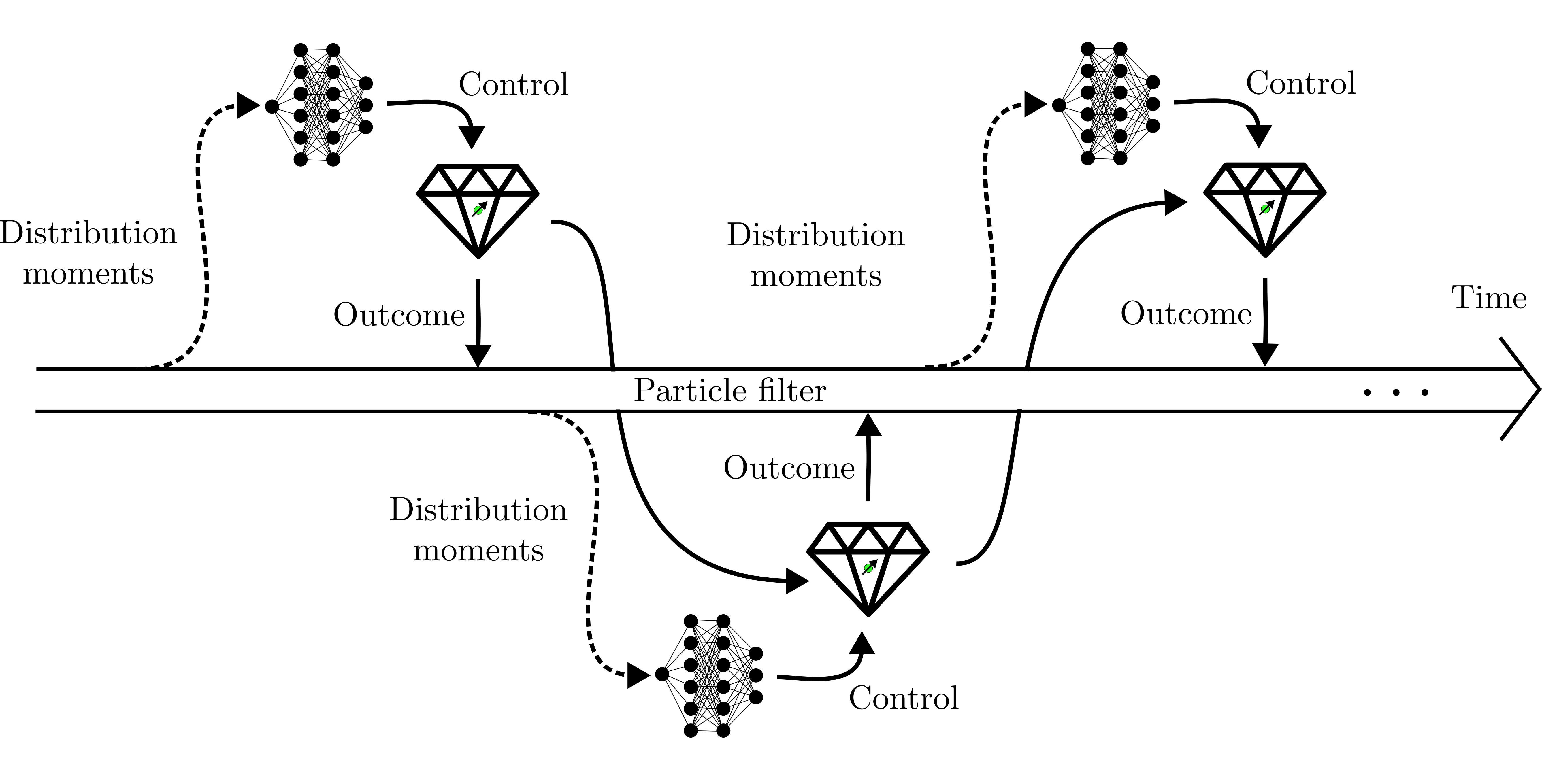

This picture represents schematically the default setting of the gradient propagation in the training. The solid arrows are the flows of information along which the gradient is propagated, while the dashed lines are the ones along which the gradient is not computed. By default the gradient is propagated along the particle filter, whose evolving state is represented by the thick blank line across the picture, along the evolving state of the probe, and through the neural network. The backpropagation of the gradient goes in the opposite direction of the information flow.

For a certain estimation in the batch we will refer to the loss produced by the method loss_function() with the symbol $\ell(\omega, \vec{\lambda})$ , with $\omega = (\vec{y}, \vec{\theta})$ , containing the list of measurement outcomes $\vec{y} = (y_0, y_2, \dots, y_{t})$ up to step $t$ , and the true values $\vec{\theta}$ of the unknown parameters to be estimated. The vector $\vec{\lambda}$ contains all the degrees of freedom of the control strategy. In case of a neural network these are the weights and the biases. The loss to be optimized is then the average of $\ell(\omega, \vec{\lambda})$ on a batch of estimations, i.e.

(17) $\mathcal{L} (\vec{\lambda}) = \frac{1}{B} \sum_{k=1}^B \ell (\omega_k, \vec{\lambda}) \;,$

where $B$ is the batchsize. If the flag cumulative_loss is deactivated the loss is computed at the end of the simulation, which is triggered when at least a fraction resources_fraction of estimations in the batch have terminated or when the maximum number of steps num_steps in the measurement loop has been achieved. If an estimation in the batch has terminated because of the resources requirements, the last estimator before the termination is used to compute the mean loss.

baseline: bool = False

If both this flag and the attribute loss_logl_outcomes are True then the loss of Eq.24 is changed to

(18) $\widetilde{\ell} (\omega, \vec{\lambda}) := \ell (\omega, \vec{\lambda})+ \text{sg}[{\ell (\omega, \vec{\lambda})} - \mathcal{B}] \log P(\vec{y}|\vec{\theta}, \vec{\lambda}) \; ,$

with

(19) $\mathcal{B} := \frac{1}{B} \sum_{k=1}^B \ell (\omega_k, \vec{\lambda}) \; ,$

The additional term should reduce the variance of the gradient computed from the batch. The baseline $\mathcal{B}$ is recomputed for each step of the measurement loop.

cumulative_loss: bool = False

With this flag on the loss of Eq.17 is computed after each measurement and accumulated, so that the quantity that is differentiated for the training at the end of the loop in execute() is

(20) $\mathcal{L}_{\text{cum}} (\vec{\lambda}) = \frac{1}{TB} \sum_{t=1}^T \sum_{k=1}^B \ell (\omega_k^t, \vec{\lambda}) \;.$

The maximum number of measurement performed is $T$ , but some estimations in the batch might terminate with less measurements. In any case the last estimator $\hat{\vec{\theta}}$ from each simulation in the batch is used to compute the mean loss in all the subsequent steps.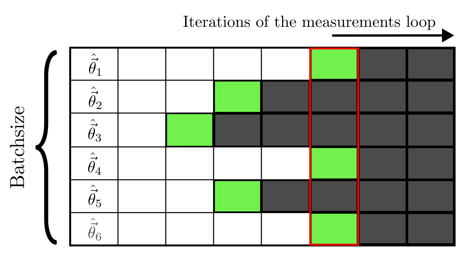

In the picture a cells of the table contains an estimator for the unknown parameters. The rows are the different simulations in the batch and the columns the steps of the measurement cycle. The current measurements step is indicated with the red box. The cells highlighted in grey are those without an estimator, either because it is not yet been computed or because the estimation is already finished for that particular batch element. In green are highlighted the $B=6$ estimators that are used in the computation of the mean loss at the current step. For the third estimation in the batch, that is already terminated, the most recent version of $\hat{\vec{\theta}}_3$ is used for computing the mean loss in all the steps after its termination.

It follows that the last estimator of those simulations that have already exhausted the resources appear multiple times in the evaluation of the loss.

Mixing precisions that refer to different number of measurements might not be a fair way to compute the loss in the metrological task. In this case the user should define the loss function so that it contains a normalization factor $\eta(\vec{\theta}_k, t)$ , that should be of the order of magnitude of the expected loss, i.e.

(21) $\frac{\ell (\omega_k^t, \vec{\lambda})}{\eta( \vec{\theta}_k, t)} \sim \mathcal{O} (1) \; .$

The cumulative loss is then

(22) $\mathcal{L}_{\text{cum}} (\vec{\lambda}) = \frac{1}{TB} \sum_{t=1}^T \sum_{k=1}^B \frac{\ell (\omega_k^t, \vec{\lambda})}{\eta(\vec{\theta}_k, t)} \;.$

Achtung! This flag has no effect on a BoundSimulation object. For which the Fisher information on the probe trajectory is already a sort of cumulative loss.

log_loss: bool = False: If this flag is True, then the used loss is the logarithm of $\mathcal{L} (\vec{\lambda})$ in Eq.17. In this case, if the flags loss_logl_controls and loss_logl_outcomes are also activated, the simulation modifies accordingly the log-likelihood terms to account for the extra logarithm in the definition of the loss. This flag can be used in conjunction with cumulative_loss to weight in the precisions at all steps in the training, while avoiding the use of a reference precision $\eta$ . The cumulative logarithmic loss would be

(23) $\mathcal{L}_{\text{log}} (\vec{\lambda}) = \frac{1}{T} \sum_{t=0}^{T-1} \log \left[ \frac{1}{B} \sum_{k=1}^B \ell (\omega_k^t, \vec{\lambda}) \right] \; .$

loss_logl_controls: bool = False

If one ore more controls are discrete, that is, their flag continuous of the Control class is False, then they are probably extracted stochastically from a probability distribution produced by the control strategy. If this is a neural network for example, its output could be the categorical distribution from which the controls are extracted, instead of the controls themselves. In such cases the callable attribute control_strategy of the Simulation class takes as input the random number generator rangen alongside input_tensor and returns controls and log_prob_control, respectively the values of the controls and the logarithm of the probability of having extracted the said values.

If this flag is True, then log_prob_control is mixed with the loss to compute the correct gradient. This means that an extra terms analogous to the one in Eq.24 is added to the loss, which refers to the controls instead of the outcomes.

This option should be activated only if the controls are generated stochastically.

loss_logl_outcomes: bool = True

If True the logarithm of the likelihood of the observed measurement outcomes is mixed with the loss $\ell(\omega, \vec{\lambda})$ in order to compute the correct gradient. The modified loss is

(24) $\widetilde{\ell} (\omega, \vec{\lambda}) := \ell (\omega, \vec{\lambda})+ \text{sg}[{\ell (\omega, \vec{\lambda})}] \log P(\vec{y}|\vec{\theta}, \vec{\lambda}) \; .$

The additional term is needed in order to propagate the gradient through the physical model of the probe, described by the differentiable methods perform_measurement() and model(), which return the logarithm of the probability of the outcomes. Without this extra term the gradient used in the training is biased. This flag must be deactivated only when the measurement outcomes are generated through a differentiable reparametrization. That is, instead of extracting $y$ directly from $P(y|\vec{\theta}, \vec{\lambda})$ it is obtained as $y=f_{\vec{\theta}, \vec{\lambda}}(z)$ , with $z$ being a stochastic variable extracted from a distribution independent on $\vec{\theta}$ and $\vec{\lambda}$ .

max_resources: float: Strict upper bound on the number of resources usable in an estimation, as counted by the count_resources() method. This parameter enters in the stopping condition of the measurement loop.

num_steps: int: Maximum number of steps in the measurement cycle of the execute() method in the Simulation class.

permutation_invariant: bool = False: If the model is invariant under permutations in the unknown parameters (for all the values of the controls) this flag should be activated. Given the unknown parameters $\theta_i$ , the ambiguity is lifted by fixing $\theta_1<\theta_2<\cdots<\theta_d$ .

prec: str = 'float64'

Floating point precision of used in the simulation, can be either float32 or float64.

Achtung! The type of the probe state defined in the attribute state_specifics of the class PhysicalModel can be different from prec, but the precisions of the ParticleFilter, PhysicalModel, SimulationParameters objects, and of the neural network should all agree.

resources_fraction: float = 1.0

Fraction of the estimations in a batch that must have exhausted the available resources for the measurement loop to stop and the batch of estimations to be declared complete. For example if resources_fraction=0.9 then only 90% of the estimations in the batch need to be terminated to stop the measurement loop of the execute() method. This parameter should be used when some of the possible simulation trajectories take a large number of measurements to saturate max_resources. Thanks to this attribute, the simulation will be stopped prematurely even if not all the estimations have terminated according to the resource availability.

Achtung! The mean loss is computed also with those estimations that have been prematurely stopped.

sim_name: str: Name of the simulation. It is the first part of the name of the files saved by the functions train(), train_nn_graph(), train_nn_profiler(), store_input_control(), and performance_evaluation()

stop_gradient_input: bool = True: Stops the propagation of the gradient through the inputs of the neural network (or in general of the control strategy). This contribution to the gradient is usually redundant, and can be neglected to spare time and memory during the training. In the picture of the SimulationParameters class description the stopping of the gradient is represented by the dashed line going from the particle filter the input of the neural network

stop_gradient_pf: bool = False

Stops the propagation of the gradient propagation through the Bayesian updates of the particle filter performed by the apply_measurement() method and represented by the thick blank line in the picture in the description of the SimulationParameters class. It can be used in conjunction with log_loss and cumulative_loss to obtain a fully greedy optimization analogous to that of the library optbayesexpt 6.

6: https://github.com/usnistgov/optbayesexpt

simulation

Module containg the Simulation class.

class Simulation(particle_filter: ParticleFilter, phys_model: PhysicalModel, control_strategy: Callable, input_size: int, input_name: List[str], simpars: SimulationParameters)

Bases: object

This is a blueprint class for all the Bayesian estimations.

Achtung! The user should not derive this class, but instead StatefulSimulation or StatelessSimulation, according to the physical model of the probe.

Attributes

bs: int: Batchsize of the simulation, i.e. number of Bayesian estimations performed simultaneously. It is taken from the phys_model attribute.
phys_model: PhysicalModel: Parameter phys_model passed to the class constructor.
control_strategy: Callable: Parameter control_strategy passed to the class constructor.
pf: ParticleFilter: Parameter particle_filter passed to the class constructor.
input_size: int: Parameter input_size passed to the class constructor.
input_name: List[str]: Parameter input_name passed to the class constructor.
simpars: SimulationParameters: Parameter simpars passed to the class constructor.
ns: int: Maximum number of steps of the measurement loop in the execute() method. It is the num_steps attribute of simpars.

Parameters passed to the Simulation class constructor.

Parameters

particle_filter: ParticleFilter

Particle filter responsible for the update of the Bayesian posterior on the parameters and on the state of the probe. It contains the methods for applying the Bayes rule and computing Bayesian estimators from the posterior.

phys_model: PhysicalModel

Abstract description of the physical model of the quantum probe. It contains the method perform_measurement() that simulates the measurement on the probe.

control_strategy: Callable

Callable object (normally a function or a lambda function) that computes the values of the controls for the next measurement from the Tensor input_strategy, which is produced by the method generate_input() defined by the user. The Simulation class expects a callable with the following header

controls = control_strategy(input_strategy)

However, if at least one of the controls is discrete, then the expected header for control_strategy is

controls, log_prob_control = control_strategy(input_strategy, rangen)

That means that some stochastic operations can be performed inside the function, like the extraction of the discrete controls from a probability distribution. The parameter rangen is the random number generator while log_prob_control is the log-likelihood of sampling the selected discrete controls.

input_size: int

Size of the last dimension of the input_strategy object passed to the callable attribute control_strategy and returned by the user-defined method generate_input(). It is the number of scalars that the function generating the controls (a neural network typically) takes as input.

input_name: List[str]

List of names for each of the scalar inputs returned by the user-defined method generate_input(). The length of input_name should be input_size. This list of names is used in the function store_input_control(), that saves a history of every input to the neural network, in order for the user to be able to interpret the actions of the optimized control strategy.

simpars: SimulationParameters

Contains the flags and parameters that regulate the stopping condition of the measurement loop and modify the loss function used in the training.

execute(rangen: Generator, deploy: bool = False)

Measurement loop and loss evaluation.

This method codifies the interaction between the sensor, the particle filter and the neural network. It contains the measurement loop schematically represented in the figure.

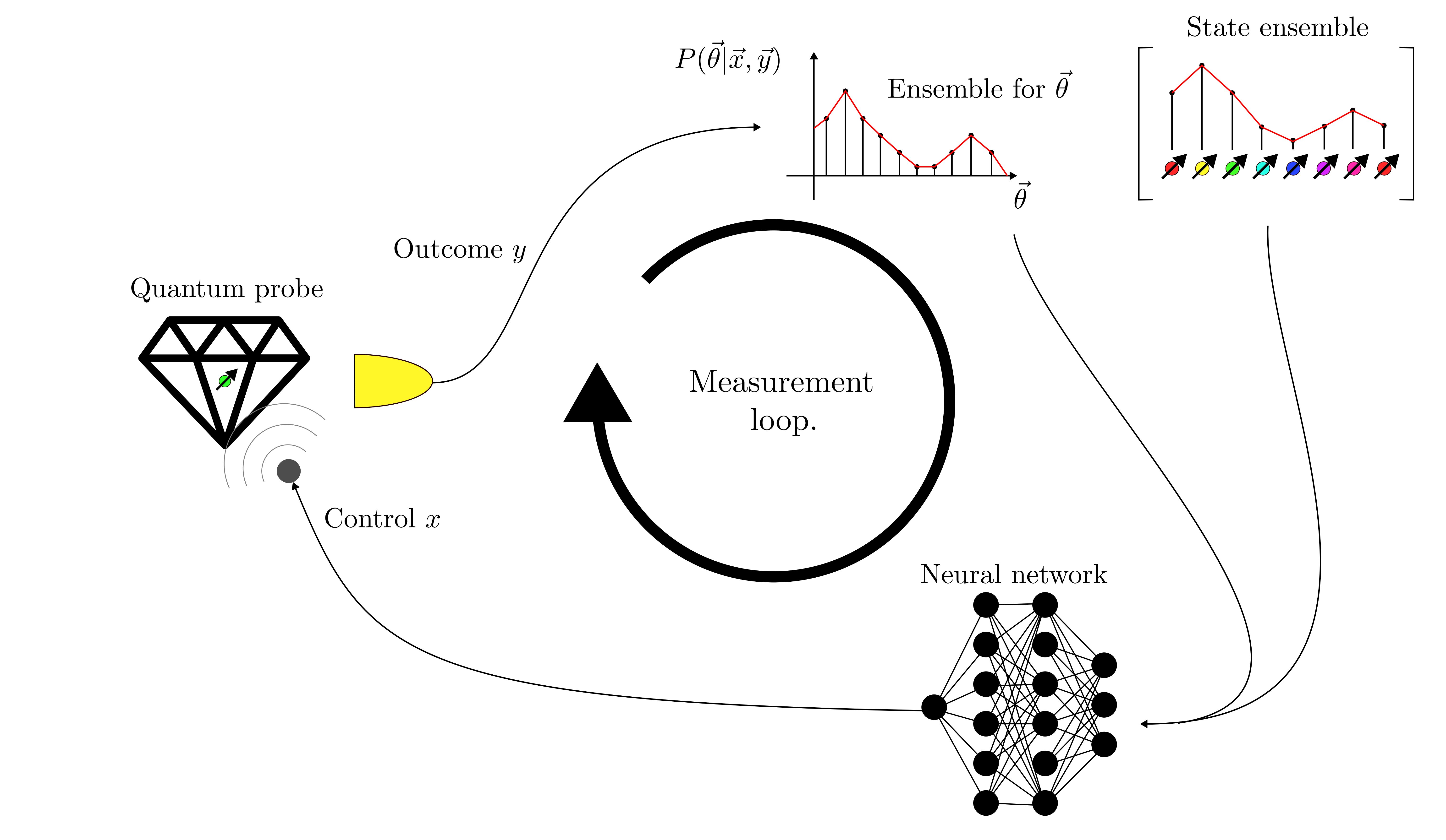
When this method is executed in the context of a GradientTape, the return value loss_diff can be differentiated with respect to the Variable objects of the control strategy for training purposes. It can also be used to evaluate the performances of a control strategy without training it. For this use, setting deploy=True is particularly useful, since it lets the method return the history of the input to the neural network, of the controls, of the consumed resources, and of the precision (the used-defined loss). This methods is used in the functions train() and performance_evaluation().

Achtung! Ideally the user never needs to use directly this method; the functions of the utils module should suffice.

The simulation of the metrological task is performed in a loop (called the measurement loop) which stops when the maximum number of iterations num_steps (called measurement steps) is reached or when the strict upper bound max_resources on the amount of resources has been saturated, as computed by the method count_resources()

Parameters

rangen: Generator: Random number generator from the module tensorflow.random.
deploy: bool: If this flag is True, the function doesn’t return the loss_diff parameter, but in its place the four histories history_input, history_control, history_resources, and history_precision.

Returns

loss_diff: Tensor

Tensor of shape (,) and type prec containing the mean value of the loss on the batch of estimations performed in the measurement loop. This is the quantity to be differentiated if the execute() method is called inside a GradientTape. This produces an unbiased estimator of the gradient of the precision for the strategy training. This version of the loss has been mixed with the log-likelihood terms for the measurement outcomes and/or the controls, according to the flags of the simpars attribute of the Simulation class, which is an instance of the SimulationParameters class. It is the mean loss as written in Eq.24 (or in Eq.18 if there is a baseline)

Achtung! This Tensor is returned only if the deploy flag passed to execute() is False.

loss: Tensor

Tensor of shape (,) and type prec containing the mean value of the loss on the batch of estimations without the mixing with the log-likelihood terms. It is the “pure” version of the mean loss computed from the user define method loss_function() and takes into account the modifying flags cumulative_loss and log_loss. This scalar is not suitable to be the differentiated loss and it is only meant to be a reference value of the true loss during the gradient descent updates that uses instead loss_diff. This return value is used in the function train() that produces, along with the trained strategy, the history of the mean losses during the training. This value is returned independently on the parameter deploy.

history_input: Tensor

Tensor of shape (ns, bs, input_size) of type prec, where ns, bs, and input_size are attributes of the Simulation class. It contains all the objects input_strategy generated by the user-defined method generate_input() and passed to the control_strategy attribute of the Simulation class, for a single call of the execute() method, for all the estimations in the batch separately and all the steps of the measurement loop. For the measurement steps that are not performed because the estimation has already run out of resources the history_input is filled with zeros.

Achtung! This Tensor is returned only if the deploy flag passed to execute() is True.

history_controls: Tensor

Tensor of shape (ns, bs, phys_model.controls_size) of type prec, where ns, bs, and phys_model are attributes of the Simulation class. It contains all the controls returned by the callable attribute control_strategy of the Simulation class, for a single call of the execute() method, for all the estimations in the batch separately and all the steps of the measurement loop. For the measurement steps that are not performed because the estimation has already run out of resources history_controls is filled with zeros.

Achtung! This Tensor is returned only if the deploy flag passed to execute() is True.

history_resources: Tensor

Tensor of shape (ns, bs, 1) of type prec, where ns, bs are attributes of the Simulation class. It contains the used resources accumulated during the estimation, as computed by the user-defined method count_resources(), for a single call of the execute() method, for all the estimations in the batch separately and all the steps of the measurement loop. For the measurement steps that are not performed because the estimation has already run out of resources history_resources is filled with zeros.

Achtung! This Tensor is returned only if the deploy flag passed to execute() is True.

history_precision: Tensor

Tensor of shape (ns, bs, 1) of type prec, where ns, bs are attributes of the Simulation class. It contains the loss as computed by the user-defined method loss_function(), for a single call of the execute() method for all the estimations in the batch separately and all the steps of the measurement loop. For the measurement steps that are not performed because the estimation has already run out of resources history_precision is filled with zeros.

Achtung! This Tensor is returned only if the deploy flag passed to execute() is True.

stateful_simulation

Module containing the StatefulSimulation class.

class StatefulSimulation(particle_filter: ParticleFilter, phys_model: PhysicalModel, control_strategy: Callable, input_size: int, input_name: List[str], simpars: SimulationParameters)

Bases: Simulation

Simulation class to be derived if the quantum probe is stateful.

If the class chosen for the model description of the probe is StatefulPhysicalModel, then StatefulSimulation is the class to be derived for describing the simulation.

Achtung! It is technically possible to have two different instances of the PhysicalModel class passed to the ParticleFilter and to the Simulation objects in their respective constructors, one being stateful and the other not. For example, one might have a stateful simulation with a stateful physical model object while the physical model of the particle filter is stateless. This means that the simulation is going to take into account the evolving state of the probe in sampling the measurement outcomes but the particle filter is unable to keep track of the states ensemble of the probe. This can be done to save memory in the training at the expense of precision.

Parameters passed to the Simulation class constructor.

Parameters

particle_filter: ParticleFilter

phys_model: PhysicalModel

Abstract description of the physical model of the quantum probe. It contains the method perform_measurement() that simulates the measurement on the probe.

control_strategy: Callable

controls = control_strategy(input_strategy)

However, if at least one of the controls is discrete, then the expected header for control_strategy is

controls, log_prob_control = control_strategy(input_strategy, rangen)

input_size: int

input_name: List[str]

simpars: SimulationParameters

Contains the flags and parameters that regulate the stopping condition of the measurement loop and modify the loss function used in the training.

generate_input(weights: Tensor, particles: Tensor, state_ensemble: Tensor, meas_step: Tensor, used_resources: Tensor, rangen) → Tensor

Computes from the particle filter ensemble and the states ensemble the input to the control_strategy attribute of the Simulation class.

Achtung! This method must be implemented by the user.

Parameters

weights: Tensor: A Tensor of weights for the particles and states ensembles with shape (bs, pf.np) and type prec. Here, pf, bs, and prec are attributes of Simulation.
particles: Tensor: A Tensor with shape (bs, pf.np, pf.d) and type prec containing the particles of the ensemble. Here, pf, bs, and prec are attributes of Simulation.
state_ensemble: Tensor: The state of the quantum probe associated with each entry of particles. Each entry of state_ensemble is the state of the probe computed as if the particles of the ensemble were the true values of the unknown parameters. It is a Tensor of shape (bs, pf.np, pf.state_size) and type pf.state_type, where pf and bs are attributes of Simulation.
meas_step: Tensor: The index of the current measurement on the probe system. The counting starts from zero. It is a Tensor of shape (bs, 1) and of type prec. bs is the attribute of the Simulation class.
used_resources: Tensor: A Tensor of shape (bs, 1) containing the total amount of consumed resources for each estimation in the batch up to the point this method is called. bs is the attribute of the Simulation class. The resources are counted according to the user defined method count_resources() from the attribute phys_model of the Simulation class.
rangen: Generator: A random number generator from the module tensorflow.random.

Returns

input_strategy: Tensor: Tensor of shape (bs, input_size), where bs and input_size are attributes of the Simulation class. This is the Tensor passed as a parameter to the call of control_strategy, which is an attribute of the Simulation class. From the elaboration of this input the function control_strategy (which is typically a wrapper for a neural network) produces the controls for the next measurement.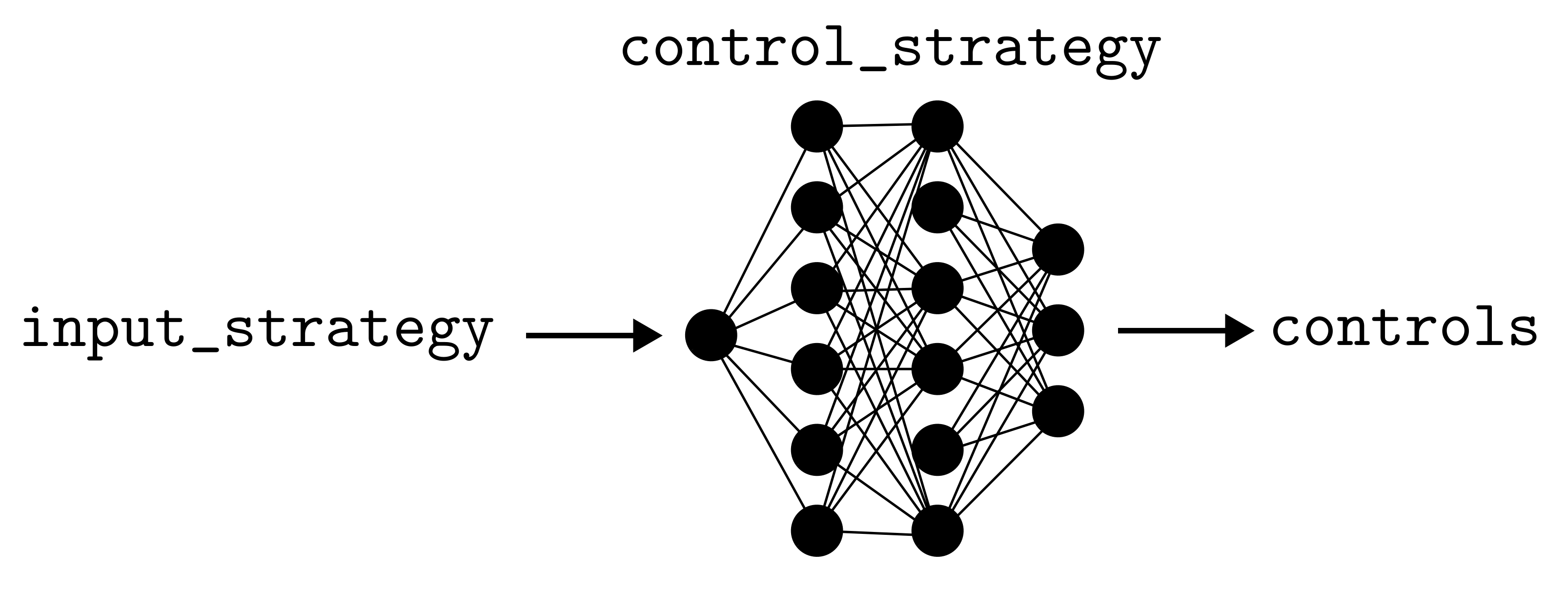

loss_function(weights: Tensor, particles: Tensor, true_state: Tensor, state_ensemble: Tensor, true_values: Tensor, used_resources: Tensor, meas_step: Tensor) → Tensor

Returns the loss to minimize in the training.

Achtung! This method has to be implemented by the user.

The loss should be the error of the metrological task, so that minimizing it in the training means optimizing the precision of the sensor. This function must return a loss value for each estimation in the batch. The actual quantity that is differentiated in the the gradient update depends also on the flags of the simpars attribute of Simulation, which is an instance of SimulationParameters. Typically the loss define by the user in this method is mixed with the log-likelihood of the of the observed outcomes in the simulation in order to obtain a bias-free estimator for the gradient from the batch.

Parameters

weights: Tensor: A Tensor of weights for the particles and states ensembles with shape (bs, pf.np) and type prec. Here, pf, bs, and prec are attributes of Simulation.
particles: Tensor: A Tensor with shape (bs, pf.np, pf.d) and type prec containing the particles of the ensemble. Here, pf, bs, and prec are attributes of Simulation.
true_states: Tensor: The true unobservable state of the probe in the estimation, computed from the evolution determined (among other factors) by the encoding of the parameters true_values. This is a Tensor of shape (bs, 1, pf.state_size), where bs and pf are attributes of the Simulation class. Its type is pf.state_type.
state_ensemble: Tensor: The state of the quantum probe associated with each entry of particles. Each entry of state_ensemble is the state of the probe computed as if the particles of the ensemble were the true values of the unknown parameters. It is a Tensor of shape (bs, pf.np, pf.state_size) and type pf.state_type, where pf and bs are attributes of Simulation.
true_values: Tensor: Contains the true values of the unknown parameters in the simulations. The loss is in general computed by comparing a suitable estimator to these values. It is a Tensor of shape (bs, 1, pf.d) and type prec, where bs, pf, and prec are attributes of the Simulation class.
used_resources: Tensor: A Tensor of shape (bs, 1) containing the total amount of consumed resources for each estimation in the batch up to the point this method is called. bs is the attribute of the Simulation class. The resources are counted according to the user defined method count_resources() from the attribute phys_model of the Simulation class.
meas_step: Tensor: The index of the current measurement on the probe system. The counting starts from zero. It is a Tensor of shape (bs, 1) and of type int32. bs is the attribute of the Simulation class.

Returns

loss_values: Tensor: Tensor of shape (bs, 1) and type prec containing the metrological error defined by the used for each estimation in the batch. bs and prec are attributes of the Simulation class.

stateless_simulation

Module containing the StatelessSimulation class.

class StatelessSimulation(particle_filter: ParticleFilter, phys_model: PhysicalModel, control_strategy: Callable, input_size: int, input_name: List[str], simpars: SimulationParameters)

Bases: Simulation

Simulation class to be derived if the quantum probe is stateless.

If the class chosen for the model description of the probe is StatelessPhysicalModel, then StatelessSimulation is the class to be derived for describing the simulation.

Parameters passed to the Simulation class constructor.

Parameters

particle_filter: ParticleFilter

phys_model: PhysicalModel

Abstract description of the physical model of the quantum probe. It contains the method perform_measurement() that simulates the measurement on the probe.

control_strategy: Callable

controls = control_strategy(input_strategy)

However, if at least one of the controls is discrete, then the expected header for control_strategy is

controls, log_prob_control = control_strategy(input_strategy, rangen)

input_size: int

input_name: List[str]

simpars: SimulationParameters

Contains the flags and parameters that regulate the stopping condition of the measurement loop and modify the loss function used in the training.

generate_input(weights: Tensor, particles: Tensor, meas_step: Tensor, used_resources: Tensor, rangen) → Tensor

Computes from the particle filter ensemble the input to the control_strategy attribute of the Simulation class.

Achtung! This method has to be implemented by the user.

Parameters

weights: Tensor: A Tensor of weights for the particle filter ensemble with shape (bs, pf.np) and type prec. Here, pf, bs, and prec are attributes of Simulation.
particles: Tensor: A Tensor with shape (bs, pf.np, pf.d) and type prec containing the particles of the ensemble. Here, pf, bs, and prec are attributes of Simulation.
meas_step: Tensor: The index of the current measurement on the probe system. The counting starts from zero. It is a Tensor of shape (bs, 1) and of type prec. bs is the attribute of the Simulation class.
used_resources: Tensor: A Tensor of shape (bs, 1) containing the total amount of consumed resources for each estimation in the batch up to the point this method is called. bs is the attribute of the Simulation class. The resources are counted according to the user defined method count_resources() from the attribute phys_model of the Simulation class.
rangen: Generator: A random number generator from the module tensorflow.random.

Returns

input_strategy: Tensor: Tensor of shape (bs, input_size), where bs and input_size are attributes of the Simulation class. This is the Tensor passed as a parameter to the call of control_strategy, which is an attribute of the Simulation class. From the elaboration of this input the function control_strategy (which is typically a wrapper for a neural network) produces the controls for the next measurement.

loss_function(weights: Tensor, particles: Tensor, true_values: Tensor, used_resources: Tensor, meas_step: Tensor) → Tensor

Returns the loss to minimize in the training.

Achtung! This method has to be implemented by the user.

Parameters

weights: Tensor: A Tensor of weights for the particle filter ensemble with shape (bs, pf.np) and type prec. Here, pf, bs, and prec are attributes of Simulation.
particles: Tensor: A Tensor with shape (bs, pf.np, pf.d) and type prec containing the particles of the ensemble. Here, pf, bs, and prec are attributes of Simulation.
true_values: Tensor: Contains the true values of the unknown parameters in the simulations. The loss is in general computed by comparing a suitable estimator to these values. It is a Tensor of shape (bs, 1, pf.d) and type prec, where bs, pf, and prec are attributes of the Simulation class.
used_resources: Tensor: A Tensor of shape (bs, 1) containing the total amount of consumed resources for each estimation in the batch up to the point this method is called. bs is the attribute of the Simulation class. The resources are counted according to the user defined method count_resources() from the attribute phys_model of the Simulation class.
meas_step: Tensor: The index of the current measurement on the probe system. The counting starts from zero. It is a Tensor of shape (bs, 1) and of type int32. bs is the attribute of the Simulation class.

Returns

loss_values: Tensor: Tensor of shape (bs, 1) and type prec containing the metrological error defined by the used for each estimation in the batches. bs and prec are attributes of the Simulation class.

bound_simulation

Module containing the BoundSimulation class, for optimizing the Cramér-Rao bound for an arbitrary estimation task.

class BoundSimulation(phys_model: PhysicalModel, control_strategy: Callable, simpars: SimulationParameters, cov_weight_matrix: Optional[List] = None, importance_sampling: bool = False, random: bool = False)

Bases: object

This simulation optimizes the Cramér-Rao bound (based on the Fisher information matrix) for the local estimation of the parameters specified in the PhysicalModel object. This class is used for frequentist inference, instead of Simulation which applies to Bayesian inference.

The Cramér-Rao bound (CR bound) is a lower bound on the Mean Square Error (MSE) matrix of the frequentist estimator $\hat{\vec{\theta}}$ at the position $\vec{\theta}$ . In formula

(25) $\Sigma_{ij} = \mathbb{E} \left[ (\hat{\vec{\theta}} - \vec{\theta})_i (\hat{\vec{\theta}} - \vec{\theta})_j \right] \ge (F^{-1})_{ij} \; ,$

in other words it codifies the maximum achievable precision of an estimator around $\vec{\theta}$ , that is, the ability to distinguish reliably two close values $\vec{\theta}$ and $\vec{\theta}+\delta \vec{\theta}$ . In the above formula we didn’t write explicitly the dependence of the estimator $\hat{\vec{\theta}} (\vec{x}, \vec{y})$ on the outcomes $\vec{y}$ and controls $\vec{x}$ trajectories of the experiment in order not to make the notation too heavy. The expectation value is taken on many realizations of the experiment, i.e. on the probability distribution of the trajectories. On the right side of Eq.25 the Fisher information matrix (FI matrix) appears, which is defined as following

(26) $F_{ij} = \mathbb{E} \left[ \frac{\partial}{\partial \theta_i} \log p(\vec{y}|\vec{\theta}, \vec{x}) \cdot \frac{\partial} {\partial \theta_j} \log p(\vec{y}|\vec{\theta}, \vec{x}) \right] \; ,$

being $p(\vec{y}|\vec{\theta}, \vec{x})$ the probability of the observed trajectory of outcomes at the point $\vec{\theta}$ . Also in this case the expectation value is taken on the experiment realizations. A scalar value for the precision is typically build from the matrix $\Sigma_{ij}$ by contracting it with a positive semidefinite weight matrix $G$ , that is the attribute cov_weight_matrix_tensor of BoundSimulation, this gives the scalar CR bound:

(27) $\text{tr} (G \cdot \Sigma_{ij}) \ge \text{tr} ( G \cdot F^{-1}) := \mathcal{L}(\vec{\lambda})\; .$

This scalar value is the loss to be minimized in the training. Let us indicate with $\vec{\lambda}$ the parameters of the control strategy (the weights and biases of a neural network), then the derivative of the loss with respect to them can be written as

(28) $\frac{\partial \mathcal{L}} {\partial \vec{\lambda}} = \text{tr} \left( F^{-1} G F^{-1} \cdot \frac{\partial F}{\partial \vec{\lambda}} \right) \; .$

The expectation value in the definition of $F$ is approximated in the simulation by averaging the product of the derivatives log-likelihoods in the batch, i.e.

(29) $F \simeq \hat{F} = \frac{1}{B}\sum_{k=1}^{B} \frac{\partial}{\partial \theta_i} \log p(\vec{y}_k|\vec{\theta}, \vec{x}_k) \cdot \frac{\partial}{\partial \theta_j} \log p(\vec{y}_k|\vec{\theta}, \vec{x}_k) = \frac{1}{B} \sum_{k=1}^B f_k \; .$

where $(\vec{x}_k, \vec{y}_k)$ is the trajectory of a particular realization of the experiment in the batch of simulations and $f_k$ is the observed Fisher information. The unbiased gradient of the FI matrix, that takes into account also the gradient of the probability distribution in the expectation value, can be computed as following

(30) $\frac{\partial \mathcal{L}} {\partial \vec{\lambda}} \simeq \frac{1}{B} \frac{\partial} {\partial \vec{\lambda}} \text{tr} \Big \lbrace \text{sg} \left( \hat{F}^{-1} G \hat{F}^{-1} \right) \sum_{k=1}^B \left[ f_k + \text{sg} (f_k) \log p(\vec{y}, \vec{x}|\vec{\theta}) \right] \Big \rbrace \; .$

The $\text{sg} (\cdot)$ is the stop_gradient operator, and the probability $p(\vec{y}, \vec{x}|\vec{\theta})$ is the likelihood of the particular trajectory, that contains both the probability of the stochastic outcome and the probability of the control (in case it is stochastically generated).

By activating the flag log_loss the loss function becomes

(31) $\mathcal{L}_{\text{log}} (\vec{\lambda}) = \log \text{tr} ( G \cdot F^{-1}) \; ,$

this is particularly useful to stabilize the training when the CR bounds spans multiple orders of magnitude.

For minimizing the CR bound around the point $\vec{\theta}$ the Parameter objects in phys_model should be initialized with the parameter values equal to the tuple containing a single element, that is the value of the parameter at the estimation point. For example the estimation around the point $\theta=0$ can be set with the following code

Parameter(values=(0.0, ), name='Theta')

This would correspond to a delta-like prior for the parameter Theta. If a different prior $\pi(\vec{\theta})$ is used, for example a uniform prior in a range, realized through the parameter bounds of the Parameter constructor, then the FI matrix approximated by the simulation is

(32) $\bar{F} = \int F (\vec{\theta}) \pi (\vec{\theta}) d \vec{\theta} \; ,$

and the minimized loss is

(33) $\text{tr} \left[ G \cdot \bar{F}^{-1} \right] \le \int \text{tr} \left( G \cdot F^{-1} (\vec{\theta}) \right) d \vec{\theta} \; ,$

which is a lower bound on the expectation value of the CR bound, because of the Jensen inequality applied to the matrix inverse. In the case of a single parameter the training maximizes the expected value of the Fisher information on the prior $\pi(\theta)$ .

With the parameter importance_sampling it is possible to use a custom distribution for extracting the trajectory. See the documentation of the class constructor for more details.

Notes

We can use this class also for the optimization of unitary quantum controls on a systems, where the only measurement is performed at the end.

Attributes

bs: int

Batchsize of the simulation, i.e. number of Bayesian estimations performed simultaneously. It is taken from the phys_model attribute.

phys_model: PhysicalModel

Parameter phys_model passed to the class constructor.

control_strategy: Callable

Parameter control_strategy passed to the class constructor.

simpars: SimulationParameters

Parameter simpars passed to the class constructor.

ns: int

Maximum number of steps of the measurement loop in the execute() method. It is the num_steps attribute of simpars.

input_size: int

Size of the last dimension of the input_strategy object passed to the callable attribute control_strategy and generated by the method generate_input(). It is the number of scalars on which control_strategy bases the prediction for the next control. By default it is computed in the constructor of the class as

input_size = d+state_size+outcomes_size+2

where d is the number of parameters to be estimated. See also the documentation of the generate_input() method.

input_name: List[str]

List of names for each of the scalar inputs returned by the method generate_input().

The list input_name contains the following elements:

The name of the d parameters in phys_model.parameters. These are d elements.
The strings “State_#, one for each scalar component of the state of the physical model. These are state_size entries.
The strings “Outcome_#”, one for each scalar outcome. These are phys_model.outcomes_size elements.
The strings “Step” and “Res”, referring respectively to the index of the measurement and the consumed resources.

This list of names is used in the function store_input_control(), that saves a history of every input to the neural network, in order for the user to be able to interpret the actions of the optimized control strategy. See also the documentation of the generate_input() method.

cov_weight_matrix_tensor: Tensor

Tensorial version of the parameter cov_weight_matrix passed to the class constructor. It is a Tensor of shape (bs, d, d) and of type prec that contains bs repetitions of cov_weight_matrix. In case no cov_weight_matrix is passed to the constructor, cov_weight_matrix_tensor contains bs copies of the d-dimensional identity matrix.

discrete_controls: bool

This flag is True if at least one of the controls is stochastically generated in the control_strategy function.

random: bool = False

Flag random passed to the class constructor.

importance_sampling: bool = False

Flag importance_sampling passed to the class constructor.

Parameters passed to the BoundSimulation class constructor.

Parameters

phys_model: PhysicalModel

Abstract description of the physical model of the quantum probe. It contains the method perform_measurement() that simulates the measurement on the probe.

control_strategy: Callable

Callable object (normally a function or a lambda function) that computes the values of the controls for the next measurement from the Tensor input_strategy, which is produced by the method generate_input(). The BoundSimulation class expects a callable with the following header

controls = control_strategy(input_strategy)

However, if at least one of the controls is discrete, then the expected header for control_strategy is

controls, log_prob_control = control_strategy(input_strategy, rangen)

simpars: SimulationParameters

Contains the flags and parameters that regulate the stopping condition of the measurement loop and modify the loss function used in the training.

cov_weight_matrix: List, optional

Weight matrix for the multiparametric estimation problem. It should be a (d, d) list, with d being the number of estimation parameters. If this parameter is not passed the default value of the weight matrix is the identity.

random: bool = False

Append a random number to the input_strategy Tensor produced by generate_input() for each element in phys_model.controls.

importance_sampling: bool = False

It is possible to implement the method perform_measurement() so that is extracts an outcome not from the true probability determined by the Born rule on the state of the probe, called $p(y|\vec{\theta}, \vec{x})$ , but from an arbitrary modified distribution $\widetilde{p}(y|\vec{\theta}, \vec{x})$ . As long as the probability implemented in the method model() is the correct one, the class BoundSimulation will be able to perform the CR bound optimization. The trajectory of the system is sampled according to $\widetilde{p}$ , and the FI matrix is computed as

(34) $F = \mathbb{E}_{\widetilde{p}} \left[ \frac{\partial}{\partial \theta_i} \log p(\vec{y}|\vec{\theta}, \vec{x}) \cdot \frac{\partial}{\partial \theta_j} \log p(\vec{y}|\vec{\theta}, \vec{x}) \frac{p(\vec{y}|\vec{\theta}, \vec{x})} {\widetilde{p}(\vec{y}|\vec{\theta}, \vec{x})} \right]$

which can be approximated on a batch as

(35) $F \simeq \frac{1}{B} \sum_{k=1}^B f_k \frac{p(\vec{y}_k|\vec{\theta}, \vec{x}_k)} {\widetilde{p}(\vec{y}_k|\vec{\theta}, \vec{x}_k)}$

with $f_k$ defined in Eq.29. Also the gradient of $F$ is changed accordingly.

Typically the distribution $\widetilde{p}$ is some perturbation of $p$ , for example it can be obtained by mixing $p$ with a uniform distribution on the outcomes.

The importance sampling is useful when some trajectories have vanishingly small probability of occurring according to the model $p$ but contribute significantly to the Fisher information. If these trajectories have some probability of occurring sampling with $\widetilde{p}$ , then the estimator of the FI might be more accurate.

The drawback is that the perturbed probability of the complete trajectory $\widetilde{p}(\vec{y}|\vec{\theta}, \vec{x})$ might be too different from the real probability (because of the accumulation of the perturbation at each step), so that the simulation might entirely miss the region in the space of trajectories in which the system state moves, thus delivering a bad estimate of the Fisher information and a bad control strategy, upon completion of the training. Whether or not the importance sampling can be beneficial to the optimization should be checked case by case.

execute(rangen: Generator, deploy: bool = False)

Measurement loop and Fisher information computation.

This method codifies the interaction between the sensor and the neural network (NN). It contains the measurement loop inside a GradientTape object used to compute the Fisher information matrix. This is done by taking the derivatives of the trajectory log-likelihood with respect to the parameters to estimate.

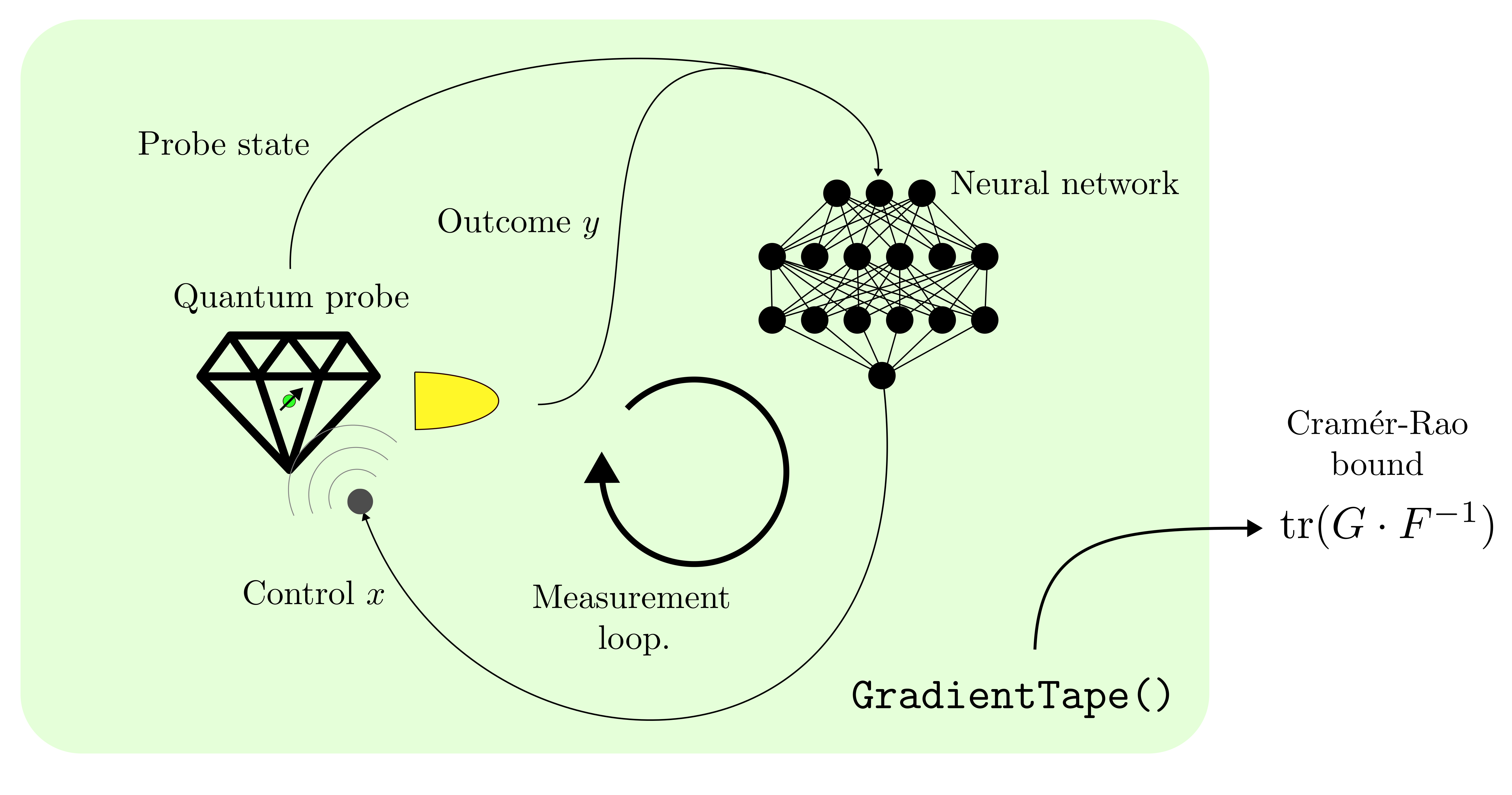
When this method is executed in the context of an external GradientTape, the return value loss_diff can be differentiated with respect to the Variable objects of the control strategy for training purposes. It can also be used to evaluate the performances of a control strategy without training it. For this use, setting deploy=True is particularly useful, since it lets the method return the history of the input to the neural network, of the controls, of the consumed resources, and of the Cramér-Rao bound for each step of the measurement loop. This methods is used in the functions train() and performance_evaluation().

Achtung! Ideally the user never needs to use directly this method; the functions of the utils module should suffice.

Parameters

rangen: Generator: Random number generator from the module tensorflow.random.
deploy: bool: If this flag is True, the function doesn’t return the loss_diff parameter, but in its place the four histories history_input, history_control, history_resources, and history_precision.

Returns

loss_diff: Tensor

Tensor of shape (,) and type prec containing the differentiable loss estimated on the batch of simulations. It is the quantity to be differentiated if the execute() method is called inside a GradientTape. This produces an unbiased estimator of the gradient of the CR bound to be used in the training. To compute loss_diff the CR bound has been mixed with the log-likelihood terms for the measurement outcomes and/or the controls, according to the flags of the simpars attribute of the BoundSimulation class, which is an instance of the SimulationParameters class. In formula it is the argument of the gradient in Eq.30.

Achtung! This Tensor is returned only if the deploy flag passed to execute() is False.

loss: Tensor

Tensor of shape (,) and type prec containing the estimator of the CR computed from $\hat{F}$ , defined in Eq.29. If log_loss is true, the loss is Eq.31. This scalar is not suitable to be differentiated and it is only meant to be a reference value of the true loss during the gradient descent updates that uses instead loss_diff. This return value is used in the function train() that produces, along with the trained strategy, the history of the mean losses during the training. This value is returned independently on the parameter deploy.

history_input: Tensor

Tensor of shape (ns, bs, input_size) of type prec, where ns, bs, and input_size are attributes of the BoundSimulation class. It contains all the objects input_strategy generated by the method generate_input() and passed to the control_strategy attribute of the BoundSimulation class, for a single call of the execute() method, for all the estimations in the batch separately and all the steps of the measurement loop. For the measurement steps that are not performed because the estimation has already run out of resources the history_input is filled with zeros.

Achtung! This Tensor is returned only if the deploy flag passed to execute() is True.

history_controls: Tensor

Tensor of shape (ns, bs, phys_model.controls_size) of type prec, where ns, bs, and phys_model are attributes of the BoundSimulation class. It contains all the controls returned by the callable attribute control_strategy of the BoundSimulation class, for a single call of the execute() method, for all the estimations in the batch separately and all the steps of the measurement loop. For the measurement steps that are not performed because the estimation has already run out of resources history_controls is filled with zeros.

Achtung! This Tensor is returned only if the deploy flag passed to execute() is True.

history_resources: Tensor

Tensor of shape (ns, bs, 1) of type prec, where ns, bs are attributes of the BoundSimulation class. It contains the used resources accumulated during the estimation, as computed by the user-defined method count_resources(), for a single call of the execute() method, for all the estimations in the batch separately and all the steps of the measurement loop. For the measurement steps that are not performed because the estimation has already run out of resources history_resources is filled with zeros.

Achtung! This Tensor is returned only if the deploy flag passed to execute() is True.

history_precision: Tensor

Tensor of shape (ns, bs, 1) of type prec, where ns, bs are attributes of the BoundSimulation class. It contains the CR bound for a single call of the execute() method for all the steps of the measurement loop. In the second dimension the values of this object are repeated. For the measurement steps that are not performed because the estimation has already run out of resources history_precision is filled with zeros.

Achtung! This Tensor is returned only if the deploy flag passed to execute() is True.

generate_input(true_values: Tensor, true_state: Tensor, meas_step: Tensor, used_resources: Tensor, outcomes: Tensor, rangen: Generator)

Constructs the input of control_strategy on the basis of which the next controls are predicted (possibly adaptively).

Achtung! If the user desires a different input_strategy Tensor he can redefine this method in a child class of BoundSimulation.

Parameters

true_values: Tensor: Contains the true values of the unknown parameters at which the Fisher information and the Cramér-Rao bound should be computed. It is a Tensor of shape (bs, 1, phys_model.d) and type prec, where bs, pf, and prec are attributes of the BoundSimulation class.
true_states: Tensor: Contains the state of the quantum probe at the current time for all the estimations in the batch. The stochastic evolution induced by perform_measurement() causes the trajectories of the state of the system to diverge. This is a Tensor of shape (bs, 1, state_size), where bs and state_size are attributes of the BoundSimulation class. Its type is state_type.
meas_step: Tensor: The index of the current measurement on the probe system. The counting starts from zero. It is a Tensor of shape (bs, 1) and of type prec. bs is the attribute of the BoundSimulation class.
used_resources: Tensor: A Tensor of shape (bs, 1) containing the total amount of consumed resources for each estimation in the batch up to the point this method is called. bs is the attribute of the BoundSimulation class. The resources are counted according to the user defined method count_resources() from the attribute phys_model of the BoundSimulation class.
outcomes: Tensor: Outcomes of the last measurement on the probe, generated by the method perform_measurement(). It is a Tensor of shape (bs, 1, phys_model.outcomes_size) of type prec.
rangen: Generator: A random number generator from the module tensorflow.random.

Return

Tensor:

Tensor of shape (bs, input_size) and type prec, with its columns being in order

true_values normalized in [-1, +1], that is, the lowest possible value of each parameter is mapped to -1 and the greates to +1. If only a single value is admissible for the parameter, then its corresponding column contains a series of ones.
true_state, i.e. the unnormalized state of phys_model at the moment this function is called.
outcomes, the unnormalized outcomes of the last measurement.
meas_step normalized in [-1, +1]
used_resources normalized in [-1, +1]
d columns of random number uniformly extracted in [0, 1], where d is the number of parameters to estimate. This column is present only if random=True.

stateful_metrology

Module containing the StatefulMetrology class

class StatefulMetrology(particle_filter: ParticleFilter, phys_model: PhysicalModel, control_strategy: Callable, simpars: SimulationParameters, cov_weight_matrix: Optional[List] = None)

Bases: StatefulSimulation

Simulation class for the standard Bayesian metrological task, with a stateful probe.

This class describes a typical metrological task, where the estimator $\hat{\vec{\theta}}$ for the unknown parameters is the mean value of the parameters on the Bayesian posterior distribution, computed with the method compute_mean(). The loss implemented in loss_function() is the mean square error (MSE) between this estimator and the true values of the unknowns used in the simulation.

The input to the neural network, computed in the method generate_input(), is a Tensor obtained by concatenating at each step the estimators for the unknown parameters, their standard deviations, their correlation matrix, the total number of consumed resources, the measurement step, and the mean of the probe state on the posterior distribution. All this variables are reparametrized/rescaled to make them fit in the [-1, 1] interval, this makes them more suitable to be the inputs of a neural network.

Achtung! The type of the probe state defined in the state_specifics attribute of the PhysicalModel class must be real.

Attributes

bs: int

Batchsize of the simulation, i.e. number of Bayesian estimations performed simultaneously. It is taken from the phys_model attribute.

phys_model: PhysicalModel

Parameter phys_model passed to the class constructor.

control_strategy: Callable

Parameter control_strategy passed to the class constructor.

pf: ParticleFilter

Parameter particle_filter passed to the class constructor.

input_size: int

Automatically generated size of the input_strategy Tensor returned by the method generate_input(). Given d the number of unknown parameters, the value of input_size is given by the following formula:

input_size = d**2+2*d+2+state_size

where state_size is the number of scalars needed to represent the state of the probe.

input_name: List[str]

List of names for each scalar entry of the input_strategy Tensor generate by generate_input().

simpars: SimulationParameters

Parameter simpars passed to the class constructor.

ns: int

Maximum number of steps of the measurement loop in the execute() method. It is the num_steps attribute of simpars.

cov_weight_matrix_tensor: Tensor

Tensor version of the parameter cov_weight_matrix passed to the class constructor. It is Tensor of shape (bs, d, d) and of type prec that contains bs repetitions of the parameter cov_weight_matrix passed to the class constructor. In case no cov_weight_matrix is passed to the constructor this Tensor contains bs copies of the d-dimensional identity matrix.

Parameters passed to the constructor of the StatefulMetrology class.

Parameters

particle_filter: ParticleFilter

phys_model: PhysicalModel

Abstract description of the physical model of the quantum probe. It contains the method perform_measurement() that simulates the measurement on the probe.

control_strategy: Callable

controls = control_strategy(input_strategy)

However, if at least one of the controls is discrete, then the expected header for control_strategy is

controls, log_prob_control = control_strategy(input_strategy, rangen)

simpars: SimulationParameters

Contains the flags and parameters that regulate the stopping condition of the measurement loop and modify the loss function used in the training.

cov_weight_matrix: List, optional

Weight matrix $G$ appearing in the computation of the loss performed by the method loss_function(). When passed, this parameter must be a List with d rows and d columns, where d is the number of parameters to estimate. It must represent a positive semidefinite matrix. This matrix controls how the errors for the multiple parameters are weighted in the scalar loss used in the weight update step. It regulates whether a parameter is of interest or is a nuisance. If this parameter is not passed then the default weight matrix is the identity, i.e. $G=\text{Id}$ .

generate_input(weights: Tensor, particles: Tensor, state_ensemble: Tensor, meas_step: Tensor, used_resources: Tensor, rangen: Generator) → Tensor

Returns the input tensor for control_strategy computed by concatenating the first moments of particle filter ensemble together with the mean state of the probe according to the Bayesian posterior, the used resources, and the measurement step.

Parameters

weights: Tensor: A Tensor of weights for the particles and states ensembles with shape (bs, pf.np) and type prec. Here, pf, bs, and prec are attributes of Simulation.
particles: Tensor: A Tensor with shape (bs, pf.np, pf.d) and type prec containing the particles of the ensemble. Here, pf, bs, and prec are attributes of Simulation.
state_ensemble: Tensor: The state of the quantum probe associated with each entry of particles. Each entry of state_ensemble is the state of the probe computed as if the particles of the ensemble were the true values of the unknown parameters. It is a Tensor of shape (bs, pf.np, pf.state_size) and type pf.state_type, where pf and bs are attributes of Simulation.
meas_step: Tensor: The index of the current measurement on the probe system. The counting starts from zero. It is a Tensor of shape (bs, 1) and of type int32. bs is the attribute of the Simulation class.
used_resources: Tensor: A Tensor of shape (bs, 1) containing the total amount of consumed resources for each estimation in the batch up to the point this method is called. bs is the attribute of the Simulation class. The resources are counted according to the user defined method count_resources() from the attribute phys_model of the Simulation class.
rangen: Generator: A random number generator from the module tensorflow.random.

Returns

input_strategy: Tensor

Tensor of shape (bs, input_size), where bs and input_size are attributes of the Simulation class. This is the Tensor passed as a parameter to the call of control_strategy, which is an attribute of the Simulation class. From the elaboration of this input the function control_strategy (which is typically a wrapper for a neural network) produces the controls for the next measurement.

input_strategy is composed on order of

Mean of unknown parameters computed on the Bayesian posterior distribution represented by the particle filter ensemble (the parameters particles and weights). It is compute calling the method compute_mean() of the pf attribute. These mean values are normalized to lay in the interval [-1, 1]. This is possible since the extrema of the admissible values for each parameters are known and codified in each Parameter object. In the input_name list these inputs are called “Mean_param.name”, where param is the corresponding Parameter object. These inputs are d scalars.
Standard deviations around the mean for each parameter computed from the Bayesian posterior distribution. The method compute_covariance() is used to compute the covariance matrix of the particle filter ensemble. Calling this matrix $C$ the next d inputs for the control strategy are given by

(36) $I_j = -\frac{2}{10} \ln \sqrt{C_{jj}} - 1\; ,$

being $\sqrt{C_{jj}}$ the said standard deviations. This time, since we do not know in advance the admissible values of the covariance matrix, we cannot cast the standard deviation exactly in [-1, 1], but we can do it approximately for standard deviations in the range 1~1e-5, through the above formula. In the input_name list these inputs are called “LogDev_param.name”, where param is the corresponding Parameter object. These inputs are d scalars.
Correlation matrix between the parameters, computed as

(37) $\rho_{ij} = \frac{C_{ij}}{\sqrt{C_{ii} C_{jj}}} \; .$

This matrix doesn’t need normalization, since its entries are already in the interval [-1, 1]. The matrix $\rho_{ij}$ is flattened and each entry is added to input_strategy, and called “Corr_param1.name_param2.name”, where param1 and param2 are Parameter objects. These inputs are d**2 scalars.
The index of the measurement step meas_step for each simulation in the batch, normalized in [-1, 1]. This input is called StepOverMaxStep and is one single scalar.
The amount of consumed resources, i.e. the parameter used_resources, normalized in [-1, 1]. This input is called resOverMaxRes and is one single scalar.
The mean state of the probe, computed from state_ensemble with weights, using the method compute_mean_state(). These are additional pf.state_size additional scalar inputs, which are not normalized. In input_name they are called State_entry_{i}, where i the index of the state entries.

Summing the total number of scalar inputs we get the formula for the attribute input_size, i.e.

input_size = d**2+2*d+2+pf.state_size

loss_function(weights: Tensor, particles: Tensor, true_state: Tensor, state_ensemble: Tensor, true_values: Tensor, used_resources: Tensor, meas_step: Tensor)

Returns for each estimation in the batch the mean square error contracted with the weight matrix $G$ , i.e. teh attribute cov_weight_matrix_tensor

Parameters

weights: Tensor: A Tensor of weights for the particles and states ensembles with shape (bs, pf.np) and type prec. Here, pf, bs, and prec are attributes of Simulation.
particles: Tensor: A Tensor with shape (bs, pf.np, pf.d) and type prec containing the particles of the ensemble. Here, pf, bs, and prec are attributes of Simulation.
true_states: Tensor: The true unobservable state of the probe in the estimation, computed from the evolution determined (among other factors) by the encoding of the parameters true_values. This is a Tensor of shape (bs, 1, pf.state_size), where bs and pf are attributes of the Simulation class. Its type is pf.state_type.
state_ensemble: Tensor: The state of the quantum probe associated with each entry of particles. Each entry of state_ensemble is the state of the probe computed as if the particles of the ensemble were the true values of the unknown parameters. It is a Tensor of shape (bs, pf.np, pf.state_size) and type pf.state_type, where pf and bs are attributes of Simulation.
true_values: Tensor: Contains the true values of the unknown parameters in the simulations. The loss is in general computed by comparing a suitable estimator to these values. It is a Tensor of shape (bs, 1, pf.d) and type prec, where bs, pf, and prec are attributes of the Simulation class.
used_resources: Tensor: A Tensor of shape (bs, 1) containing the total amount of consumed resources for each estimation in the batch up to the point this method is called. bs is the attribute of the Simulation class. The resources are counted according to the user defined method count_resources() from the attribute phys_model of the Simulation class.
meas_step: Tensor: The index of the current measurement on the probe system. The counting starts from zero. It is a Tensor of shape (bs, 1) and of type int32. bs is the attribute of the Simulation class.

Returns

loss_values: Tensor: Tensor of shape (bs, 1) and type prec containing the mean square error of the mean of the posterior estimator. bs and prec are attributes of the Simulation class.

The error on the metrological estimation task is:

(38) $\mathcal{L} (\vec{\lambda}) = \text{tr} [ G \cdot \Sigma (\vec{\lambda})] \; ,$

where $\vec{\lambda}$ are the trainable variables of the control strategy (the weights and biases of the neural network), $\Sigma$ is the mean error matrix of the estimator $\hat{\vec{\theta}}$ on the batch, i.e.

(39) $\Sigma_{ij} = \sum_{k=1}^B (\hat{\vec{\theta}} - \vec{\theta})_i (\hat{\vec{\theta}} - \vec{\theta})_j \; ,$

while $G$ is a semi-positive matrix of shape (d, d) called the weight matrix that is used to obtain a scalar error in a multiparameter metrological problem. The integer d is the dimension of $\vec{\theta}$ . This matrix controls which errors contribute to the final loss and how much. It discriminates also between parameters of interest and nuisances, which do not contribute to the scalar loss $\mathcal{L}(\vec{\lambda})$ , because their corresponding entries in the $G$ matrix are null.

The mean loss in Eq.38 can be expanded as

(40) $\mathcal{L} (\vec{\lambda}) = \sum_{k=1}^B \text{tr} [G \cdot (\hat{\vec{\theta}}_k - \vec{\theta}_k)_i (\hat{\vec{\theta}}_k - \vec{\theta}_k)_j ] \; ,$

from which is clear what the loss $\ell (\omega_k, \vec{\lambda})$ for each single estimation in the batch should be:

(41) $\ell (\omega_k, \vec{\lambda}) = \text{tr} [G \cdot (\hat{\vec{\theta}}_k - \vec{\theta}_k)_i (\hat{\vec{\theta}}_k - \vec{\theta}_k)_j ] \; ,$

with $\omega_k = (\vec{y}_k, \vec{\theta}_k)$ being a tuple that contains the string of observed measurement outcomes and the true values $\vec{\theta}_k$ for a particular estimation in the batch. This is the loss implemented in this method.

stateless_metrology

Module containing the StatelessMetrology class

class StatelessMetrology(particle_filter: ParticleFilter, phys_model: PhysicalModel, control_strategy: Callable, simpars: SimulationParameters, cov_weight_matrix: Optional[List] = None)

Bases: StatelessSimulation

Simulation class for the standard Bayesian metrological task, with a steless probe.

The input to the neural network, computed in the method generate_input(), is a Tensor obtained by concatenating at each step the estimators for the unknown parameters, their standard deviations, their correlation matrix, the total number of consumed resources, and the measurement step. All this variables are reparametrized/rescaled to make them fit in the [-1, 1] interval, this makes them more suitable to be the inputs of a neural network.

Attributes

bs: int

Batchsize of the simulation, i.e. number of Bayesian estimations performed simultaneously. It is taken from the phys_model attribute.

phys_model: PhysicalModel

Parameter phys_model passed to the class constructor.

control_strategy: Callable

Parameter control_strategy passed to the class constructor.

pf: ParticleFilter

Parameter particle_filter passed to the class constructor.

input_size: int

input_size = d**2+2*d+2

input_name: List[str]

List of names for each scalar entry of the input_strategy Tensor generate by generate_input().

simpars: SimulationParameters

Parameter simpars passed to the class constructor.

ns: int

Maximum number of steps of the measurement loop in the execute() method. It is the num_steps attribute of simpars.

cov_weight_matrix_tensor: Tensor

Parameters passed to the constructor of the StatelessMetrology class.

Parameters

particle_filter: ParticleFilter

phys_model: PhysicalModel

Abstract description of the physical model of the quantum probe. It contains the method perform_measurement() that simulates the measurement on the probe.

control_strategy: Callable

controls = control_strategy(input_strategy)

However, if at least one of the controls is discrete, then the expected header for control_strategy is

controls, log_prob_control = control_strategy(input_strategy, rangen)

simpars: SimulationParameters

Contains the flags and parameters that regulate the stopping condition of the measurement loop and modify the loss function used in the training.

cov_weight_matrix: List, optional

generate_input(weights: Tensor, particles: Tensor, meas_step: Tensor, used_resources: Tensor, rangen: Generator) → Tensor

Returns the input tensor for control_strategy computed by concatenating the first moments of particle filter ensemble together with the used resources, and the measurement step.

Parameters

weights: Tensor: A Tensor of weights for the particle filter ensemble with shape (bs, pf.np) and type prec. Here, pf, bs, and prec are attributes of Simulation.
particles: Tensor: A Tensor with shape (bs, pf.np, pf.d) and type prec containing the particles of the ensemble. Here, pf, bs, and prec are attributes of Simulation.
meas_step: Tensor: The index of the current measurement on the probe system. The counting starts from zero. It is a Tensor of shape (bs, 1) and of type int32. bs is the attribute of the Simulation class.
used_resources: Tensor: A Tensor of shape (bs, 1) containing the total amount of consumed resources for each estimation in the batch up to the point this method is called. bs is the attribute of the Simulation class. The resources are counted according to the user defined method count_resources() from the attribute phys_model of the Simulation class.
rangen: Generator: A random number generator from the module tensorflow.random.

Returns

input_strategy: Tensor

input_strategy is composed on order of

Mean of unknown parameters computed on the Bayesian posterior distribution represented by the particle filter ensemble (the parameters particles and weights). It is compute calling the method compute_mean() of the pf attribute. These mean values are normalized to lay in the interval [-1, 1]. This is possible since the extrema of the admissible values for each parameters are known and codified in each Parameter object. In the input_name list these inputs are called “Mean_param.name”, where param is the corresponding Parameter object. These inputs are d scalars.
Standard deviations around the mean for each parameter computed from the Bayesian posterior distribution. The method compute_covariance() is used to compute the covariance matrix of the particle filter ensemble. Calling this matrix $C$ the next d inputs for the control strategy are given by

(42) $I_j = -\frac{2}{10} \ln \sqrt{C_{jj}} - 1 \; ,$

being $\sqrt{C_{jj}}$ the said standard deviations. This time, since we do not know in advance the admissible values of the covariance matrix, we cannot cast the standard deviation exactly in [-1, 1], but we can do it approximately for standard deviations in the range 1~1e-5, through the above formula. In the input_name list these inputs are called “LogDev_param.name”, where param is the corresponding Parameter object. These inputs are d scalars.
Correlation matrix between the parameters, computed as

(43) $\rho_{ij} = \frac{C_{ij}}{\sqrt{C_{ii} C_{jj}}} \; .$

This matrix doesn’t need normalization, since its entries are already in the interval [-1, 1]. The matrix $\rho_{ij}$ is flattened and each entry is added to input_strategy, and called “Corr_param1.name_param2.name”, where param1 and param2 are Parameter objects. These inputs are d**2 scalars.
The index of the measurement step meas_step for each simulation in the batch, normalized in [-1, 1]. This input is called StepOverMaxStep and is one single scalar.
The amount of consumed resources, i.e. the parameter used_resources, normalized in [-1, 1]. This input is called resOverMaxRes and is one single scalar.

Summing the total number of scalar inputs we get the formula for the attribute input_size, i.e.

input_size = d**2+2*d+2

loss_function(weights: Tensor, particles: Tensor, true_values: Tensor, used_resources: Tensor, meas_step: Tensor)

Parameters

weights: Tensor: A Tensor of weights for the particle filter ensemble with shape (bs, pf.np) and type prec. Here, pf, bs, and prec are attributes of Simulation.
particles: Tensor: A Tensor with shape (bs, pf.np, pf.d) and type prec containing the particles of the ensemble. Here, pf, bs, and prec are attributes of Simulation.
true_values: Tensor: Contains the true values of the unknown parameters in the simulations. The loss is in general computed by comparing a suitable estimator to these values. It is a Tensor of shape (bs, 1, pf.d) and type prec, where bs, pf, and prec are attributes of the Simulation class.
used_resources: Tensor: A Tensor of shape (bs, 1) containing the total amount of consumed resources for each estimation in the batch up to the point this method is called. bs is the attribute of the Simulation class. The resources are counted according to the user defined method count_resources() from the attribute phys_model of the Simulation class.
meas_step: Tensor: The index of the current measurement on the probe system. The counting starts from zero. It is a Tensor of shape (bs, 1) and of type int32. bs is the attribute of the Simulation class.

Returns

loss_values: Tensor: Tensor of shape (bs, 1) and type prec containing the mean square error of the mean of the posterior estimator. bs and prec are attributes of the Simulation class.

Returns for each estimation in the batch the mean square error contracted with the weight matrix $G$ , i.e. the attribute cov_weight_matrix_tensor

The error on the metrological estimation task is:

(44) $\mathcal{L} (\vec{\lambda}) = \text{tr} [ G \cdot \Sigma (\vec{\lambda})] \; ,$

(45) $\Sigma_{ij} = \sum_{k=1}^B (\hat{\vec{\theta}} - \vec{\theta})_i (\hat{\vec{\theta}} - \vec{\theta})_j \; ,$

The mean loss in Eq.44 can be expanded as

(46) $\mathcal{L} (\vec{\lambda}) = \sum_{k=1}^B \text{tr} [G \cdot (\hat{\vec{\theta}}_k - \vec{\theta}_k)_i (\hat{\vec{\theta}}_k - \vec{\theta}_k)_j ] \; ,$

from which is clear what the loss $\ell (\omega_k, \vec{\lambda})$ for each single estimation in the batch should be:

(47) $\ell (\omega_k, \vec{\lambda}) = \text{tr} [G \cdot (\hat{\vec{\theta}}_k - \vec{\theta}_k)_i (\hat{\vec{\theta}}_k - \vec{\theta}_k)_j ] \; ,$

schedulers

Module containing the InverseSqrtDecay class.

class InverseSqrtDecay(initial_learning_rate: float, prec: str = 'float64')

Bases: LearningRateSchedule

Inverse square root decay of the learning rate.

This class implements a learning rate schedule that allows the learning rate used in the training to be a function of the iteration number, that is the number of gradient descent updates of the training variables already performed. In particular, this class realize the following schedule for the learning rate $l_r(i)$ as function of the iteration number (starting from zero):

(48) $l_r(i) := \frac{l_r(0)}{\sqrt{i+1}} \; ,$

being $l_r(0)$ the initial learning rate. The reason for wanting a decay of the learning rate is to let the neural network learn finer and finer details of the optimal control strategy as the training goes on, for which smaller and smaller updated steps are needed.

Constructor of the InverseSqrtTimeDecay class.

Parameters

initial_learning_rate: float: Learning rate use in the first iteration of the training cycle (the number zero iteration).
prec: str: Floating point precision of the variable to be trained. Can be either float32 or float64.

get_config()

utils

Module containing some utility functions for training the control strategy and visualizing the results.

class FitSpecifics

Bases: TypedDict

This dictionary specifies the hyperparameters of the precision fit operated by the function performance_evaluation().

batchsize: int: Batchsize of the training of the neural network to fit the Precision/Resources relation. The data cloud is divided in minibatches and each of them is used for a sigle iteration of the training loop.

direct_func: Callable

Callable object that takes in input the precision and the consumed resources and outputs a values $x$ that is of order one. In symbols

(49) $f(\text{Resources}, \text{Precision}) = x \sim \mathcal{O}(1) \; .$

This requires having some knowledge of the expected precision given the resources, which could be for example a Cramér-Rao bound on the precision.

epochs: int: The number of trainings on the same data.

inverse_func: Callable: Inverse of the function defined by direct_func, that is

(50) $g(\text{Resources}, x) = \text{Precision} \; .$

num_points: int: After the fit the neural network representing the relation between the resources and the average precision is evaluated on num_points resources values equally spaced in the interval [0, max_resources], with max_resources being the attribute of SimulationParameters.

denormalize(input_tensor: Tensor, bounds: Tuple[float, float]) → Tensor

Given input_tensor with values in [-1, 1] this function rescales it, so that its entries take values within the given tuple of extrema.

Parameters

input_tensor: Tensor: Tensor having entries normalized in [-1, 1].
bound: Tuple[float, float]: Min and max of the admissible entries of the returned Tensor.

Returns

Tensor:

Version of input_tensor normalized in the interval delimited by the new extrema. Each entry $y$ of input_tensor becomes

(51) $x = \frac{y (\text{bound}[1]- \text{bound}[0])}{2}+\text{bounds}[0] \; .$

It is a Tensor with the same type and shape of input_tensor.

get_seed(random_generator: Generator) → Tensor

Generate a random seed from random_generator.

Extracts uniformly a couple of integers from random_generator to be used as seed in the stateless functions of the tensorflow.random module.

Parameters

random_generator: Generator: Random number generator from the module tensorflow.random.

Returns

seed: Tensor: Tensor of shape (2, ) and of type int32 containing two random seeds.

loggauss(x, mean, dev)

Logarithm of a batch of 1D-Gaussian probability densities.

Parameters

x: Tensor: Values extracted from the Gaussian distributions. Must have the same type and size of mean and dev.
mean: Tensor: Means of the Gaussian distributions. Must have the same type and size of x and dev.
dev:: Standard deviation of the Gaussian distributions. Must have the same type and size of mean and x.

Returns

Tensor:

Logarithm of the probability densities for extracting the entries of x from the Gaussian distributions defined by mean and dev. It has the same shape and type of x, mean, and dev.

Calling $x$ , $\mu$ , and $\sigma$ respectively an entry of the tensor x, mean, and dev, the corresponding entry of the returned tensor is

(52) $-\log \left( \sqrt{2 \pi} \sigma \right) - \frac{(x-\mu)^2}{2 \sigma^2} \; .$

logpoisson(mean, k)

Logarithm of the probability densities of a batch of Poissonian distributions.

Parameters

mean: Tensor: Mean values defining the Poissonian distributions. Must have the same type and shape of k.
k: Tensor: Observed outcomes of the sampling from the Poissonian distributions. Must have the same type and shape of k.

Returns

Tensor:

Tensor having the same type and shape of mean and k, whose entries are defined by

(53) $k \log (\mu) - \mu - \log (k !) \; ,$

where $k$ and $\mu$ are respectively the entries of k and mean.

normalize(input_tensor: Tensor, bounds: Tuple[float, float]) → Tensor

Normalizes the entries of input_tensor in the interval [-1, 1]. The input_tensor entries must lay within the given tuple of upper and lower bounds.

Parameters

input_tensor: Tensor: Tensor of unnormalized values.
bound: List[float, float]: Min and max of the admissible entries of input_tensor.

Returns

Tensor:

Version of input_tensor with entries normalized in the interval [-1, 1]. Each entry $x$ of the input becomes

(54) $y = \frac{2(x-\text{bound}[0])}{\text{bound}[1]- \text{bound}[0]} - 1 \;$

in the returned Tensor, which has the same type and shape of input_tensor.

npgauss_pdf(x, dev): Logarithm of a batch of 1D-Gaussian probability densities (compatible with Numpy)

performance_evaluation(simulation, iterations: int, data_dir: str, xla_compile: bool = True, precision_fit: ~typing.Optional[~qsensoropt.utils.FitSpecifics] = None, delta_resources: ~typing.Optional[float] = None, y_label: str = 'Precision', rangen=<tensorflow.python.ops.stateful_random_ops.Generator object>)

Computes the relation Precision/Resources obtained from the averaged data of a number iterations of runs of the execute() method. Such relation is saved on disk as as a list of points (Resources, Precision) in a csv file, whose name terminate with “_eval”.

The “resources” in the estimation task are defined in the method count_resources(). Different executions of the task can only be compared when they refer to the same amount of resources.

Since the estimation is a stochastic process this routine will produce the expected precision as a function of the consumed resources.

Parameters

simulation: Simulation

Contains the complete description of the estimation task, and how the various components of it (particle filter, probe system, and control) interact to produce the estimator and the loss.

iterations: int

Number of update steps in the training of the strategy. It is the number of complete executions of a batch of estimation tasks.

data_dir: str

Directory containing the csv file with the evaluated relation Precision/Resources.

xla_compile: bool = True

Just-in-time XLA (Accelerated Linear Algebra) compilation for the simulation. It should reduce the used memory and time on a GPU.

Achtung! Not all the Tensorflow operations can be compiled with XLA.

Achtung! It might not perform well on a CPU.

precision_fit: FitSpecifics, optional

The simulations produce a cloud of points (Resources, Precision) from which a simple relation between the expected precision and the resources must be obtained. One possibility is to fit this cloud of points with a neural network.

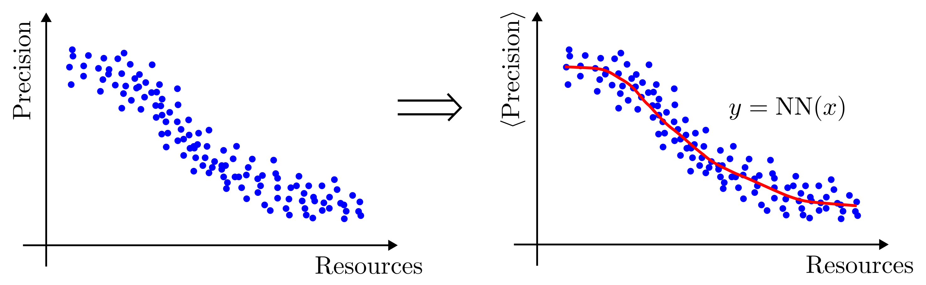
When the dictionary parameter_fit is passed to the call of this routine, then the cloud of points is fitted, and the fitted curve is saved in the csv file.

delta_resources: float, optional

The simulations produce a cloud of points (Resources, Precision), and all the points inside a window of resources of size delta_resources are averaged in order to produce a single point containing the expected precision, which is practically the barycenter of the said window.

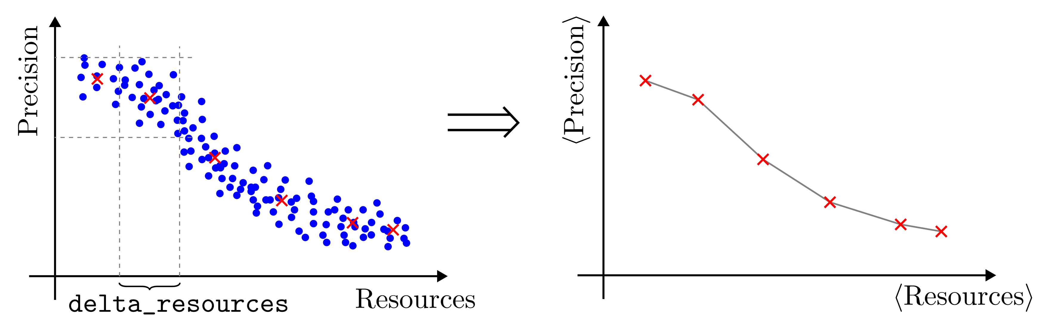
The barycenters of all the consecutive windows are saved in the csv file produced by this routine.

y_label: str = ‘Precision’

Label of the y-component of the data saved in the csv file. This column represent the precision of the estimation and more specifically it could be the the mean square error, the error probability, etc.

rangen: Generator = Generator.from_seed(0xdeadd0d0)

Random number generator from the module tensorflow.random.

Notes

The parameters precision_fit and delta_resources are not mutually exclusive. When both are passed to the call of the routine, first the cloud of (Resources, Precision) points is averaged according to the value of delta_resources and then the fewer points resulting from the averaging are fitted with a neural network.

random_uniform(batchsize: int, prec: str, min_value: float, max_value: float, seed: Tensor)

Extracts batchsize random number of type prec between the min_value and the max_value from a uniform distribution.

Parameters

batchsize: int: Number of random values to be extracted.
prec: str: Type of the extracted numbers. It is typically float32 or float64.
min_values: float: Lower extremum of the uniform distribution from which the values are extracted.
max_values: float: Upper extremum of the uniform distribution from which the values are extracted.
seed: Tensor: Seed of the random number generator used in this function. It is a Tensor of type int32 and of shape (2, ). This is the kind of seed that is accepted by the stateless random function of the module tensorflow.random. It can be generated with the function get_seed() from a Generator object.

Returns

Tensor:: Tensor of shape (batchsize, ) and of type prec with uniformly extracted entries.

sqrt_hmatrix(matrix: Tensor) → Tensor

Square root of the absolute value of a symmetric (hermitian) matrix.

The default matrix square root algorithm implemented in Tensorflow 7 doesn’t work for matrices with very small entries, this implementation does, and must be always preferred.

Parameters

matrix: Tensor: Batch of symmetric (hermitian) square matrices.

Returns

Tensor:: Matrix square root of matrix.

Examples

A = constant([[1e-16, 1e-15], [1e-15, 1e-16]], dtype="float64", )

print(tf.sqrtm(A))

Output:

[[-nan -nan], [-nan -nan]]

While print(sqrt_hmatrix(A)) outputs

[[1.58312395e-09, 3.15831240e-08], [3.15831240e-08, 1.58312395e-09]]

7: N. J. Higham, “Computing real square roots of a real matrix”, Linear Algebra Appl., 1987.

standard_model(input_size: int = 1, controls_size: int = 1, neurons_per_layer: int = 64, num_mid_layers: int = 5, prec: str = 'float64', normalize_activation: bool = True, sigma_input: float = 0.33, last_layer_activation: str = 'tanh') → Model

Returns a dense neural network to fit the optimal control strategy.

Parameters

input_size: int = 1: Number of scalars given in input to the neural network.
controls_size: int = 1: Number of scalars outputted by the neural network. It corresponds to the number of controls in the estimation task.
neurons_per_layer: int = 64: Number of units (neurons) in each intermediate layer of the neural network. The intermediate layers of the neural network are all identical.
num_mid_layers: int = 5: Number of layers between the input and the output of the neural network. Should be greater then one.
prec: str = “float64”: Type of the weights and biases of the neural network.
normalize_activation: bool = True: If this flag is active the activation function (tanh) is normalized to preserve the variance of the input after each layer of neurons. This should speed up the convergence.
sigma_input: float = 0.33: Approximate variance of the input of the neural network. The default value is the variance of a uniform distribution in [-1, +1].
last_layer_activation: str = “tanh”: Activation function of the last neural network layer.

Returns

Model:: Sequential model made up of num_mid_layers intermediate layers, each with neurons_per_layer units. The initialization of the weight and biases is done with glorot uniform and the activation function is tanh, possibly normalized to reduce the saturation.

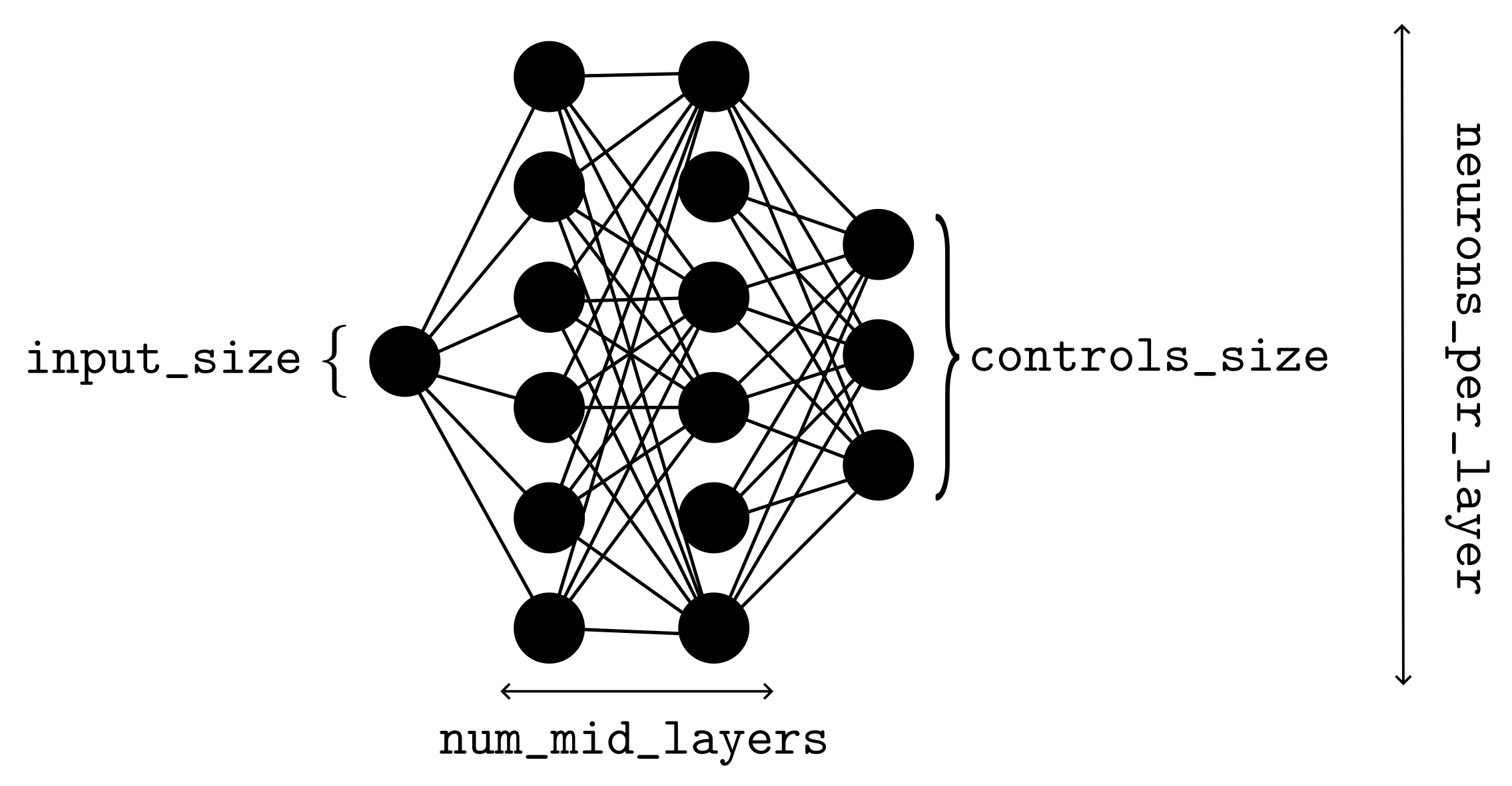
store_input_control(simulation, data_dir: str, iterations: int, xla_compile: bool = True, rangen=<tensorflow.python.ops.stateful_random_ops.Generator object>)

This routine collects data on the behavior of of the control_strategy attribute of the simulation parameter.

Stores in a csv file all the input_strategy and the controls tensors, which are respectively the input and the output of the callable attribute control_strategy of simulation, which is a Simulation object. The inputs are returned by the generate_input() method. In the produced csv file, whose name ends in “_ext.csv” the input_strategy and controls tensors for each estimation in the batch, for a number iterations of executions of the execute method.

The first column of the produced csv file is Estimation and it is the index of the independent estimation to which the line is referring. It is incremented both across the batchsize and the iterations, so that it goes from 0 to bs*iterations-1. The next d columns are the true values of the unknown parameters, where d is the attribute of simulation.ps, i.e. the ParticleFilter attribute of simulation. The next simulation.input_size columns are the entries of input_strategy produced by generate_input(). The last simulation.phys_model.controls_size columns contains the controls produced by simulation.control_strategy. The name of the columns are taken from the name attributes of the corresponding objects and from simulations.input_name.

Achtung! The lines with null consumed resources are not reported in the csv file.

Parameters

simulation: Simulation

Contains the complete description of the estimation task, and how the various components of it (particle filter, probe system, and control) interact to produce the estimator and the loss.

data_dir: str

Directory in which the csv file containing the

iterations: int

Number of update steps in the training of the strategy. It is the number of complete executions of a batch of estimation tasks for training the controls.

xla_compile: bool = True

Just-in-time XLA (Accelerated Linear Algebra) compilation for the simulation. It should reduce the used memory and time on a GPU.

Achtung! Not all the Tensorflow operations can be compiled with XLA.

Achtung! It might not perform well on a CPU.

rangen: Generator = Generator.from_seed(0xdeadd0d0)

Random number generator from the module tensorflow.random.

train(simulation, optimizer: ~keras.optimizers.optimizer.Optimizer, iterations: int, save_path: str, interval_save: int = 128, network: ~typing.Optional[~keras.engine.training.Model] = None, custom_controls: ~typing.Optional[~tensorflow.python.ops.variables.Variable] = None, load_best: bool = True, gradient_accumulation: int = 1, xla_compile: bool = True, rangen: ~tensorflow.python.ops.stateful_random_ops.Generator = <tensorflow.python.ops.stateful_random_ops.Generator object>)

Training routine for the neural network or the custom controls.

This function contains a cycle that performs a gradient descent optimization of the training variables of the control strategy.

Parameters

simulation: Simulation

Contains the complete description of the estimation task, and how the various components of it (particle filter, probe system, and control) interact to produce the estimator and the loss.

optimizer: Optimizer

This object applies the gradient to the trainable variables of the control strategy and realized therefore the update of the gradient descent step. The default optimizer to be chosen is Adam with the variable learning rate described in the class InverseSqrtDecay.

iterations: int

Number of update steps in the training of the strategy. It is the number of complete executions of a batch of estimation tasks for training the controls.

save_path: str

Path containing the intermediate trained variables, that are saved each interval_save iterations, and the history of the loss at the end of the training.

interval_save: int = 128

Number of iterations of the training cycle between two consecutive saving of the training variables on disk.

network: Model, optional

Neural network model used in the simulation object to parametrize the control strategy. In simulation it is wrapped inside the control_strategy attribute and there the Simulation object has no direct access to its trainable variables. If no neural network is used in the estimation, for example because a static strategy is being trained, this parameter can be omitted.

custom_controls: Variable, optional

It is possible to train a control strategy that goes beyond what can be done with a neural network, by writing a custom control_strategy function which is not only a wrapper for the neural network. The trainable variables of this custom strategy are contained in the object object custom_controls.

The typical application is that of a static strategy, that is a control strategy that depends only on the measurement step and not on the posterior distribution moments. This is a non-adaptive strategy, that therefore doesn’t need to be computed in real time, but can be hard coded before the beginning of the estimation. Such approach will save memory, because the Bayesian analysis can be postponed and performed on a more powerful device, and it will also be faster, because no computation is necessary between two measurements, since the approach is non-adaptive. Of course one can’t expect in general the same performances of the adaptive strategy.

load_best: bool = True

Keeps track of the loss of the control strategy during the training and picks the best model instead of the last. To pick the best model the loss is averaged over interval_save update steps.

gradient_accumulation: int = 1

This controls the “effective” batchsize of the training. In the training loop for each update of the variables the method execute() runs a number gradient_accumulation of times and the gradients computed from each run are averaged before the update step is performed. In this way, given bs the true batchsize of the simulation object, the “effective” batchsize of the training is gradient_accumulation*bs, which is the number of independent simulations that contribute to a single update step of the training variables. This feature can be used to increase the batchsize, when the memory on the machine is limited, since the maximum amount of memory required by the training is determine by bs and is independent on gradient_accumulation.

xla_compile: bool = True

Just-in-time XLA (Accelerated Linear Algebra) compilation for the strategy training. It should reduce the memory and training time on a GPU.

Achtung! Not all the Tensorflow operations can be compiled with XLA.

Achtung! It might not perform well on a CPU.

rangen: Generator = Generator.from_seed(0xdeadd0d0)

Random number generator from the module tensorflow.random.

After the return of the train() routine either network or the custom_controls will be trained and in save_path there will be a directory containing the partially trained variables (with name ending in “_weights”) and a csv file with the history of the loss (with name ending in “_history.csv”), averaged over a window of interval_save iterations.

train_nn_graph(simulation, optimizer: ~keras.optimizers.optimizer.Optimizer, data_dir: str, network, rangen=<tensorflow.python.ops.stateful_random_ops.Generator object>)

Produces a report of the tensor operations in the training that can be visualized in Tensorboard as a graph.

Achtung! This function works only for the training of a neural network.

Parameters

simulation: Simulation: Contains the complete description of the estimation task, and how the various components of it (particle filter, probe system, and control) interact to produce the estimator and the loss.
optimizer: Optimizer: This object applies the gradient to the trainable variables of the control strategy and realized therefore the update of the gradient descent step. The default optimizer to be chosen is Adam with the variable learning rate described in the class InverseSqrtDecay.
data_dir: str: Directory in which the report containing the computational graph is saved.
network: Model, optional: Neural network model used in the simulation object to parametrize the control strategy. In simulation it is wrapped inside the control_strategy attribute and there the Simulation object has no direct access to its trainable variables. If no neural network is used in the estimation, for example because a static strategy is being trained, this parameter can be omitted.
rangen: Generator = Generator.from_seed(0xdeadd0d0): Random number generator from the module tensorflow.random.

train_nn_profiler(simulation, optimizer: ~keras.optimizers.optimizer.Optimizer, data_dir: str, network: ~keras.engine.training.Model, iterations: int = 10, gradient_accumulation: int = 1, xla_compile: bool = True, rangen=<tensorflow.python.ops.stateful_random_ops.Generator object>)

Saves profiling information regarding the memory and time consumption of each operation in the simulation that can be visualized on Tensorboard.

Parameters

simulation: Simulation

Contains the complete description of the estimation task, and how the various components of it (particle filter, probe, …) interact to produce the estimator and the loss.

optimizer: Optimizer

data_dir: str

Directory in which the report on the profiling data is saved.

network: Model, optional

iterations: int = 10

Number of update steps in the training of the strategy. It is the number of complete executions of a batch of estimation tasks for training the controls.

gradient_accumulation: int = 1

xla_compile: bool = True

Just-in-time XLA (Accelerated Linear Algebra) compilation for the strategy training. It should reduce the memory and training time on a GPU.

Achtung! Not all the Tensorflow operations can be compiled with XLA.

Achtung! It might not perform well on a CPU.

rangen: Generator = Generator.from_seed(0xdeadd0d0)

Random number generator from the module tensorflow.random.

plot_utils

Module containing some useful routines for plotting the data contained in the csv file produced by the routines of the utils module. This module relies on the functionalities of the Matplotlib.

plot_2_values(df: DataFrame, x: str, y: str, figsize: Tuple[float, float] = (3.0, 2.0), dpi: float = 200.0, path: Optional[str] = None, log_scale: bool = True, log_scale_x: bool = False, vertical: bool = True)

Plots two arrays of values, in a standard 2d line plot.

Parameters

df: DataFrame: Pandas DataFrame containing the values to plot. It must have two columns named x and y respectively. This routine will plot df[y] as a function of df[x].
x: str: Name of the x-axis
y: str: Name of the y-axis.
figsize: Tuple[float, float] = (3.0, 2.0): Width and height of the figure in inches.
dpi: float = 200.0: Resolution of the figure in dots-per-inch.
path: str = None: Directory in which the figure is saved. If it is not passed, the figure is not saved on disk.
log_scale: bool = True: Logarithmic scale on the y-axis.
log_scale_x: bool = False: Logarithmic scale on the x-axis.
vertical: bool = True: Orientation of the label of the y-axis.

Notes

The name of the saved plot is plot_{x}_{y}.png.

plot_3_values(df: DataFrame, x: str, y: str, color: str, figsize: Tuple[float, float] = (3.0, 2.0), dpi: float = 200.0, path: Optional[str] = None, vertical: bool = True)

Plots three arrays of values, one encoded in the color of the point in a scatter plot.

Parameters

df: DataFrame: Pandas DataFrame containing the values to plot. It must have three columns named respectively x, y, and color. This routine will plot the tuples of points (df[x], df[y]) in a scatter plot. The color of the points is the column df[color], which must have values in [0, 1].
x: str: Name of the x-axis
y: str: Name of the y-axis.
color: str: Name of the column represented as the color of points in the scatter plot.
figsize: Tuple[float, float] = (3.0, 2.0): Width and height of the figure in inches.
dpi: float = 200.0: Resolution of the figure in dots-per-inch.
path: str = None: Directory in which the figure is saved. If it is not passed, the figure is not saved on disk.
vertical: bool = True: Orientation of the label of the y-axis.

Notes

The name of the saved plot is plot_{x}_{y}_c_{color}.png.

plot_4_values(df: DataFrame, x: str, y: str, z: str, color: str, figsize: Tuple[float, float] = (6.0, 4.0), dpi: float = 300.0, path: Optional[str] = None)

Plot four array of values in a 3d scatter plot. One of the values is encoded in the color of the points.

Parameters

df: DataFrame: Pandas DataFrame containing the values to plot. It must have four columns named respectively x, y, z, and color. This routine will plot the tuples of points (df[x], df[y], df[z]) in a 3d scatter plot. The color of the points is the column df[color], which must have values in [0, 1].
x: str: Name of the x-axis
y: str: Name of the y-axis.
z: str: Name of the z-axis.
color: str: Name of the column represented as the color of points in the scatter plot.
figsize: Tuple[float, float] = (6.0, 4.0): Width and height of the figure in inches.
dpi: float = 300.0: Resolution of the figure in dots-per-inch.
path: str = None: Directory in which the figure is saved. If it is not passed, the figure is not saved on disk.

Notes

The name of the saved plot is plot_{x}_{y}_{z}_c_{color}.png.

plot_multiples(list_df: List[DataFrame], x: str, y: str, list_labels: List[str], figsize: Tuple[float, float] = (3.0, 2.0), dpi: float = 200.0, path: Optional[str] = None, log_scale: bool = True, log_scale_x: bool = False, title: str = '', legend_location: str = 'upper right', vertical: bool = True, list_line_syles: Optional[List[str]] = None, lower_bound_df: Optional[DataFrame] = None)

Plots two arrays of values for multiple datasets, for comparison purposes, in a standard line plot.

Parameters

list_df: List[DataFrame]: List of Pandas DataFrame containing the values to plot. Each DataFrame in the list must have two columns named x and y respectively. This routine will plot df[y] as a function of df[x] for all the elements df of list_df on the same figure.
x: str: Name of the x-axis
y: str: Name of the y-axis.
list_labels: List[str]: List of labels for each DataFrame in list_df. These are the names visualized in the legend.
figsize: Tuple[float, float] = (3.0, 2.0): Width and height of the figure in inches.
dpi: float = 200.0: Resolution of the figure in dots-per-inch.
path: str = None: Directory in which the figure is saved. If it is not passed, the figure is not saved on disk.
log_scale: bool = True: Logarithmic scale on the y-axis.
log_scale_x: bool = False: Logarithmic scale on the x-axis.
title: str = “”: Title of the plot.
legend_location: str = “upper right”,: Location of the legend.
vertical: bool = True: Orientation of the label of the y-axis.
list_line_syles: List[str] = None: List of strings specifying the style for each line.
lower_bound_df: DataFrame = None: DataFrame containing the lower bound for the precision plot. Under this line everything must be colored in grey.

Notes

The name of the saved plot is plot_{x}_{y}.png.